models — Fitting models

This page documents the various fitting models readily available in the package.

Polynomials

Constant

A constant model. (Note this is equivalent to a polynomial of degree zero, but we keep it separate for clarity.)

\[f(x;~c) = c \quad \text{with} \quad c \rightarrow \texttt{value}\]

Fitting with a constant model is equivalent to computing the weighted average of the values of the dependent variable.

Line

A straight-line model. (Note this is equivalent to a polynomial of degree one, but we keep it separate for clarity.)

\[\begin{split}f(x;~m, q) = mx + q \quad \text{with} \quad \begin{cases} m \rightarrow \texttt{slope} \\ q \rightarrow \texttt{intercept} \end{cases}\end{split}\]

Polynomial

A simple polynomial model of arbitrary degree.

\[f(x;~c_0, c_1, \ldots, c_n) = \sum_{k=0}^{n} c_k x^k \quad \text{with} \quad c_k \rightarrow \texttt{c0, c1, ..., cn}\]

The degree of the polynomial is set at initialization time via the degree argument in the constructor, e.g.,

>>> quadratic = Polynomial(2)
>>> cubic = Polynomial(degree=3)

Quadratic

Simple alias for a polynomial of degree two.

Cubic

Simple alias for a polynomial of degree three.

Exponentials and power-laws

PowerLaw

A power-law model with the general form:

\[\begin{split}f(x;~N, \Gamma) = N \left(\frac{x}{x_0}\right)^\Gamma \quad \text{with} \quad \begin{cases} N \rightarrow \texttt{prefactor}\\ \Gamma \rightarrow \texttt{index}\\ x_0 \rightarrow \texttt{pivot}~\text{(set at creation time)} \end{cases}\end{split}\]

Note

The overloaded plot() method automatically switches to a log-log scale.

Exponential

A simple exponential model:

\[\begin{split}f(x;~N, X) = N \exp \left\{-\frac{(x - x_0)}{X}\right\} \quad \text{with} \quad \begin{cases} N \rightarrow \texttt{prefactor}\\ X \rightarrow \texttt{scale}\\ x_0 \rightarrow \texttt{location}~\text{(set at creation time)} \end{cases}\end{split}\]

Note

Note that the location parameter is not a fit parameter, but rather a fixed offset that is set when the model instance is created, e.g.,

>>> exponential = Exponential(location=2.0)

The basic idea behind this is to avoid the degeneracy between the location and the prefactor, and this is one of the main reasons this model is not implemented wrapping the scipy exponential distribution.

ExponentialComplement

The exponential complement, describing an exponential rise:

\[\begin{split}f(x;~N, X) = N \left [ 1- \exp\left\{-\frac{(x - x_0)}{X}\right\} \right ] \quad \text{with} \quad \begin{cases} N \rightarrow \texttt{prefactor}\\ X \rightarrow \texttt{scale}\\ x_0 \rightarrow \texttt{location}~\text{(set at creation time)} \end{cases}\end{split}\]

Note

See notes on Exponential regarding the location parameter.

StretchedExponential

A stretched exponential model:

\[\begin{split}f(x;~N, X, \gamma) = N \exp \left\{-\left[\frac{(x - x_0)}{X}\right]^\gamma\right\} \quad \text{with} \quad \begin{cases} N \rightarrow \texttt{prefactor}\\ X \rightarrow \texttt{scale}\\ \gamma \rightarrow \texttt{stretch}\\ x_0 \rightarrow \texttt{location}~\text{(set at creation time)} \end{cases}\end{split}\]

Note

See notes on Exponential regarding the location parameter.

StretchedExponentialComplement

The complement of the stretched exponential model:

\[\begin{split}f(x;~N, X, \gamma) = N \left [ 1- \exp\left\{-\left[\frac{(x - x_0)}{X}\right]^\gamma\right\} \right ] \quad \text{with} \quad \begin{cases} N \rightarrow \texttt{prefactor}\\ X \rightarrow \texttt{scale}\\ \gamma \rightarrow \texttt{stretch}\\ x_0 \rightarrow \texttt{location}~\text{(set at creation time)} \end{cases}\end{split}\]

Note

See notes on Exponential regarding the location parameter.

Models related to the gaussian

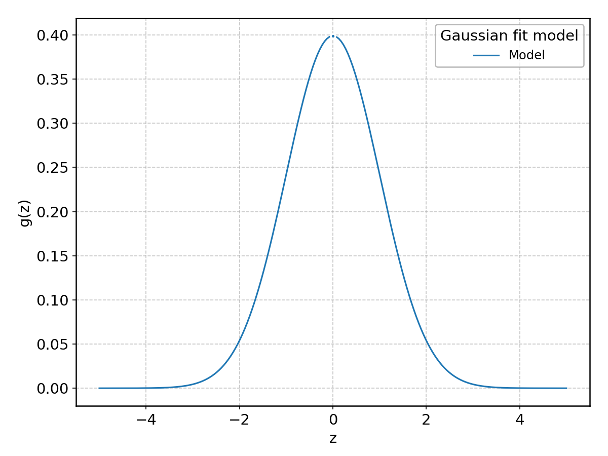
Gaussian

This is actually not wrapped from scipy.stats.norm, but rather a direct implementation of the gaussian (normal) distribution, mainly to override the parameter names.

Among other things, this class provides a method to perform an iterative fit around the peak, which is not available in the generic Normal class.

See also

The Normal is an alternative, equivalent implementation wrapping scipy.stats.norm as all the other location-scale models. Any additional features specific to the gaussian distribution will be implemented in Gaussian, so users are encouraged to use this class over Normal, except for testing purposes.

Fe55Forest

Gaussian line forest for the Kα and Kβ emission features of \(^{55}\mathrm{Fe}\) decay, using intensity-weighted mean energies from the X-ray database (<https://xraydb.seescience.org/>).

Probit

This is a custom implementation of the inverse of the cumulative distribution function (also known as the percent-point function) of a normal distribution with generic location and scale.

\[\begin{split}f(x;~\mu,~\sigma) = \mu + \sigma \Phi^{-1}(x) \quad \text{with} \quad \begin{cases} \mu \rightarrow \texttt{offset}\\ \sigma \rightarrow \texttt{sigma} \end{cases}\end{split}\]

where \(\Phi^{-1}(x)\) is the actual Probit function (the percent-point function of the standard normal distribution).

Note

For completeness, this is internally implemented using the scipy.special.ndtri() function, rather than using scipy.stats.norm.ppf(), but the two are fully equivalent.

The support of this model is the interval \(0 < x < 1\), since the Probit function diverges at the boundaries. Therefore, when plotting this model, the default plotting range is automatically set to a slightly smaller interval in order to avoid issues at the boundaries.

Note that, since the mean of the underlying normal distribution translates into a vertical shift of the Probit function, the former is called offset in this context—not mu. For completeness, the sigma parameter controls the scale of the vertical excursion of the model. Also note that we do not provide a prefactor parameter since it would be completely degenerate with the other two, and would be basically impossible to fit in a sensible way.

Sigmoid models

Sigmoid models are location-scale models defined in terms of a standardized shape function \(g(z)\)

\[f(x; A, m, s, \ldots) = A g\left(\frac{x - m}{s}; \ldots \right)\]

where \(A\) is the amplitude (total height of the sigmoid), \(m\) is the location (typically the point where the value of the function if 50% of the amplitude) and \(s\) is the scale parameter, representing the width of the transtion.

Note

In this case the amplitude parameter does not represent an area (as in peak-like models), but rather the total increase of the function from its lower asymptote to its upper asymptote.

Note when the scale parameter is negative, we switch to the complement of the sigmoid function, i.e., a monotonically decreasing function from 1 to 0 (in standard form).

\(g(z)\) is generally a monotonically increasing function, ranging from 0 to 1 as its argument goes from -infinity to +infinity, as illustrated below for some of the models available in the package.

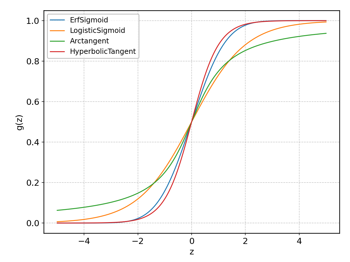
ErfSigmoid

The cumulative function of a gaussian distribution:

\[g(z) = \frac{1}{2} \left(1 + \operatorname{erf}\left(\frac{z}{\sqrt{2}}\right)\right)\]

Warning

The naming might be slightly unfortunate here, as, strictly speaking, this is not the error function defined, e.g., in scipy.special, but hopefully it is clear enough in the context of model fitting.

LogisticSigmoid

A logistic sigmoid defined by the standard shape function:

\[g(z) = \frac{1}{1 + e^{-z}}\]

Arctangent

An arctangent sigmoid defined by the standard shape function:

\[g(z) = \frac{1}{2} + \frac{1}{\pi} \arctan(z)\]

    @staticmethod
    def shape(z):
        # pylint: disable=arguments-differ
        return 0.5 + np.arctan(z) / np.pi

HyperbolicTangent

An hyperbolic tangent sigmoid defined by the standard shape function:

\[g(z) = \frac{1}{2} \left(1 + \tanh(z)\right)\]

Continuous random variables

Most of the models defined in this package are wrappers around continuous random variables defined in scipy.stats, which provide a large variety of standardized distributions. Most (but not all) of these distributions can be interpreted as peak-like models. All of them are location-scale models defined in terms of a standardized shape function \(g(z)\)

\[f(x; A, m, s, \ldots) = \frac{A}{s} g\left(\frac{x - m}{s}; \ldots \right)\]

where \(A\) is the amplitude (area under the peak), \(m\) is the location (parameter specifying the peak position), and \(s\) is the scale (parameter specifying the peak width). The trailing \ldots indicates any additional shape parameters that might be required by the specific distribution.

See also

modeling — Modeling

The rest of this section lists all the available distributions, with a brief description of their support and shape parameters. For more details on each distribution, please refer to the corresponding documentation in scipy.stats.

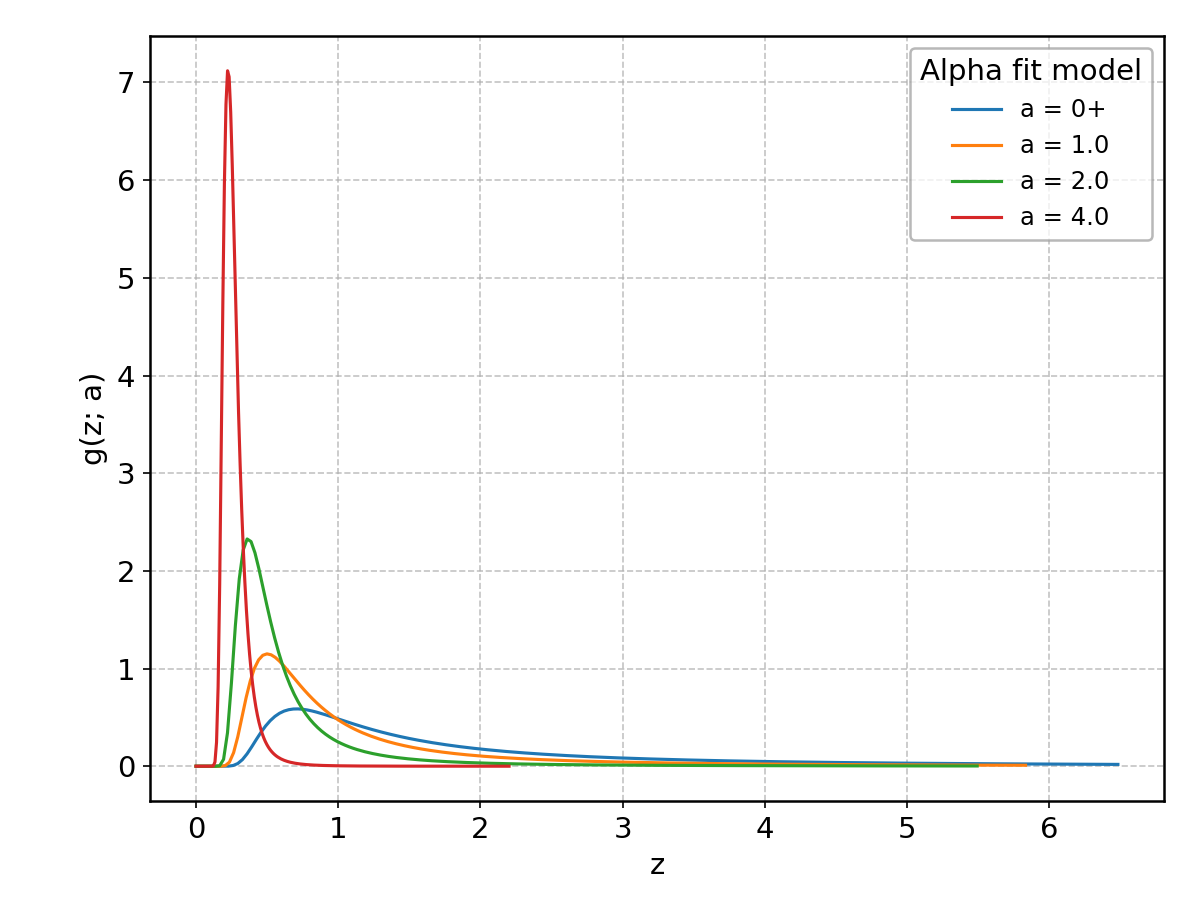
Alpha

Wrapped from scipy.stats.alpha; support: \(z > 0\); shape parameter(s): \(a > 0\).

(Note the mean and the standard deviation of the distribution are always infinite.)

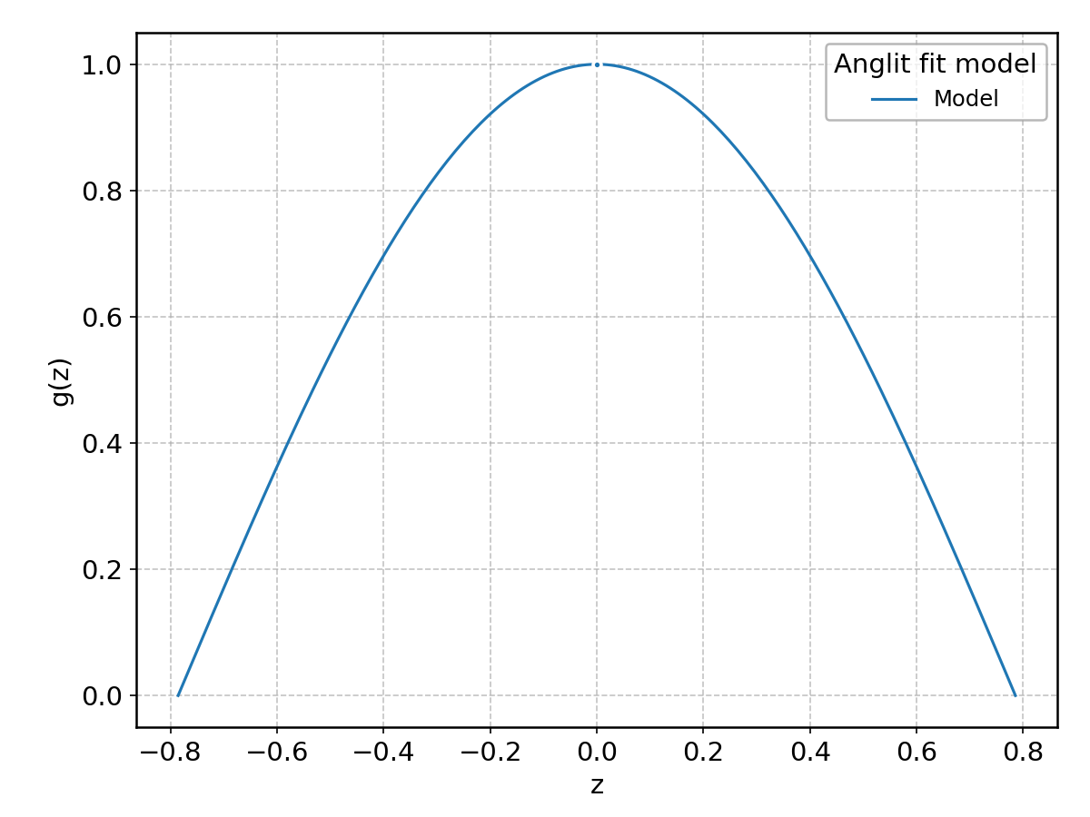
Anglit

Wrapped from scipy.stats.anglit; support: \(-\pi/4 \le z \le \pi/4\).

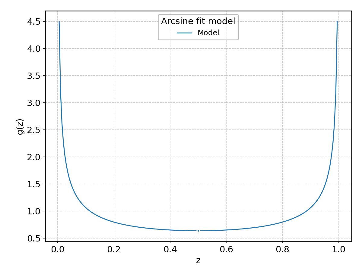
Arcsine

Wrapped from scipy.stats.arcsine; support: \(0\le z \le 1\).

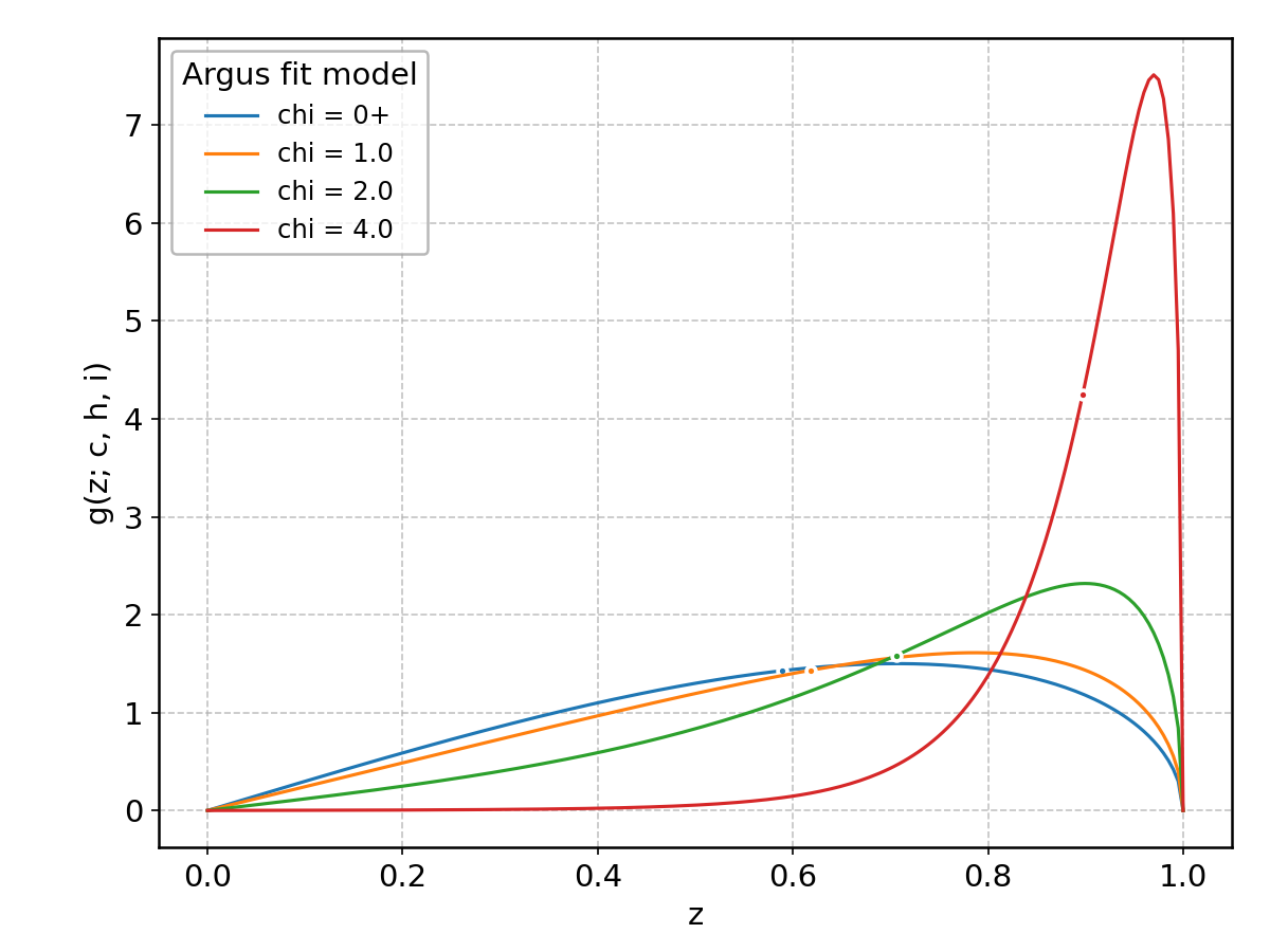
Argus

Wrapped from scipy.stats.argus; support: \(0 < z < 1\); shape parameter(s): \(\chi > 0\).

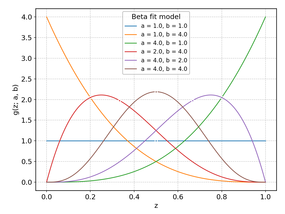
Beta

Wrapped from scipy.stats.beta; support: \(0 < z < 1\); shape parameter(s): \(a> 0\), \(b > 0\).

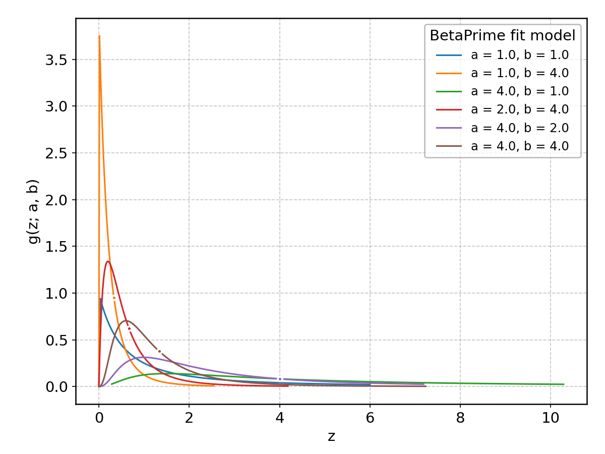
BetaPrime

Wrapped from scipy.stats.betaprime; support: \(0 < z < 1\); shape parameter(s): \(a> 0\), \(b > 0\).

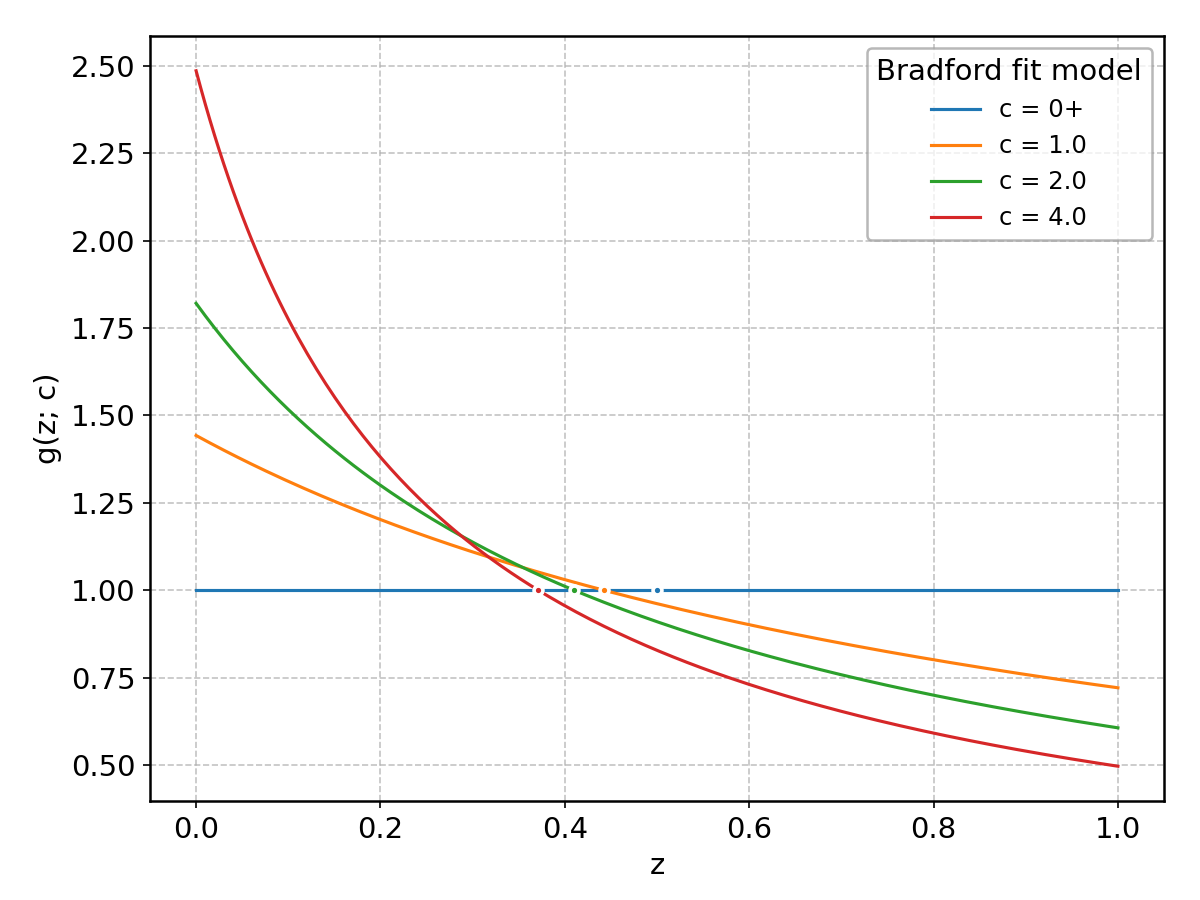
Bradford

Wrapped from scipy.stats.bradford; support: \(0 < z < 1\); shape parameter(s): \(c > 0\).

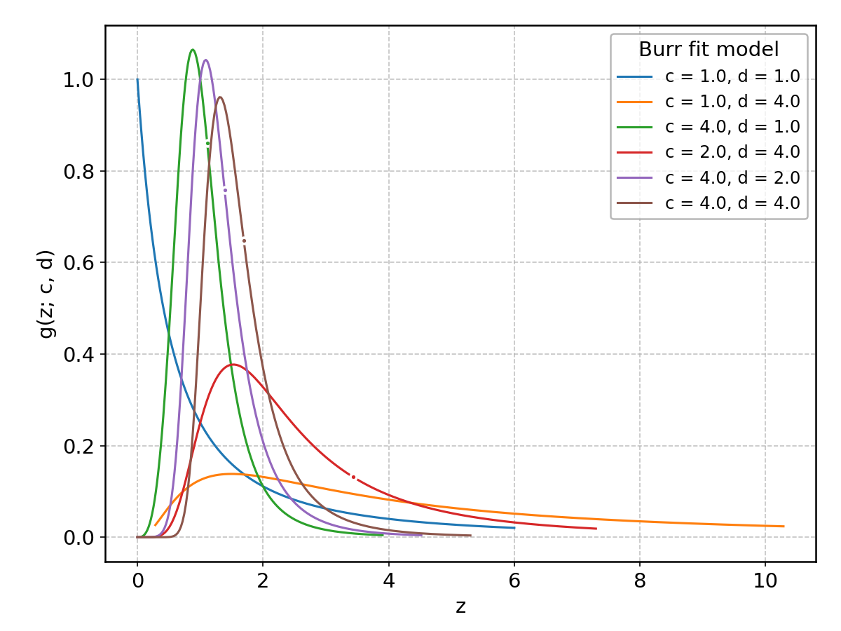
Burr

Wrapped from scipy.stats.burr; support: \(z > 0\); shape parameter(s): \(c, d > 0\).

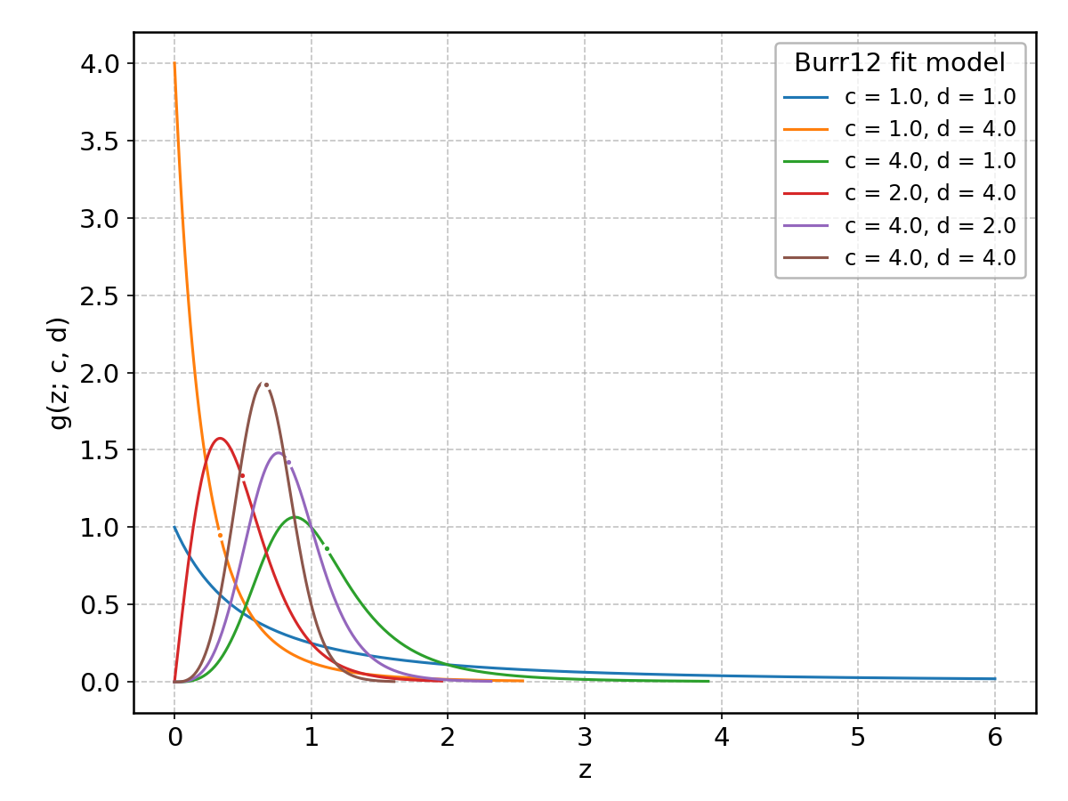
Burr12

Wrapped from scipy.stats.burr12; support: \(z > 0\); shape parameter(s): \(c, d > 0\).

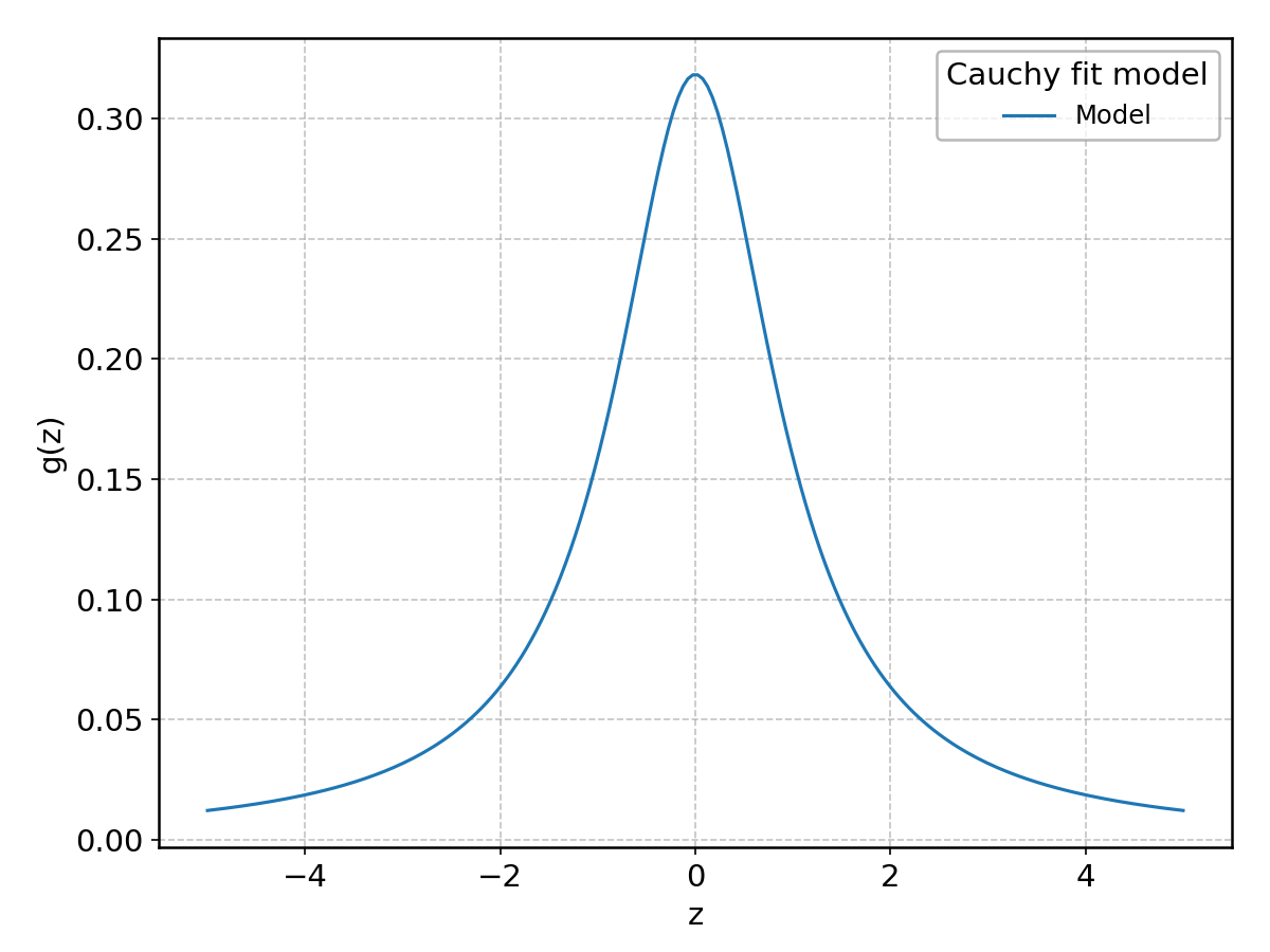
Cauchy

Wrapped from scipy.stats.cauchy; support: \(z > 0\).

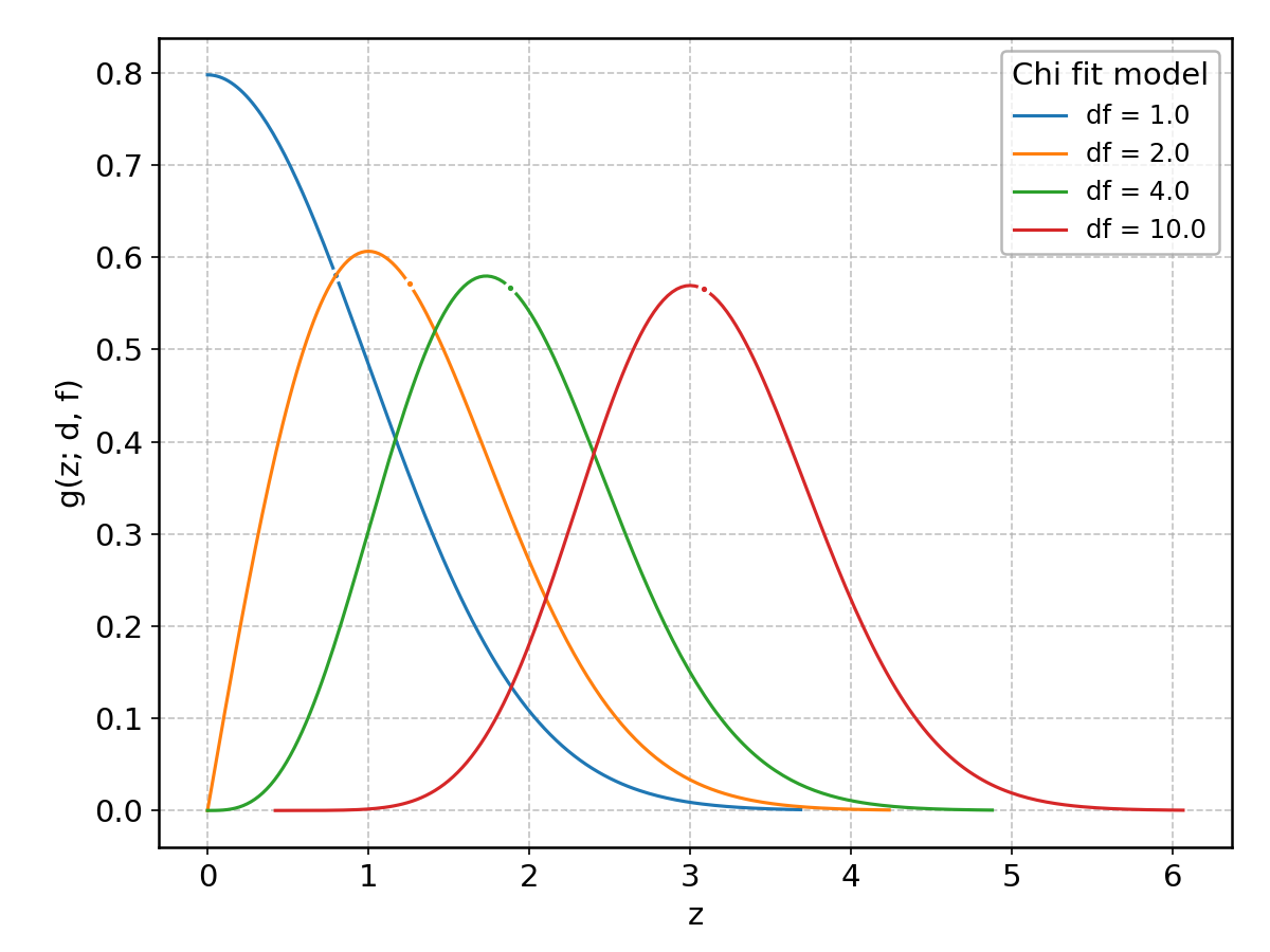
Chi

Wrapped from scipy.stats.chi; support: \(z > 0\); shape parameter(s): \(\text{df} > 0\).

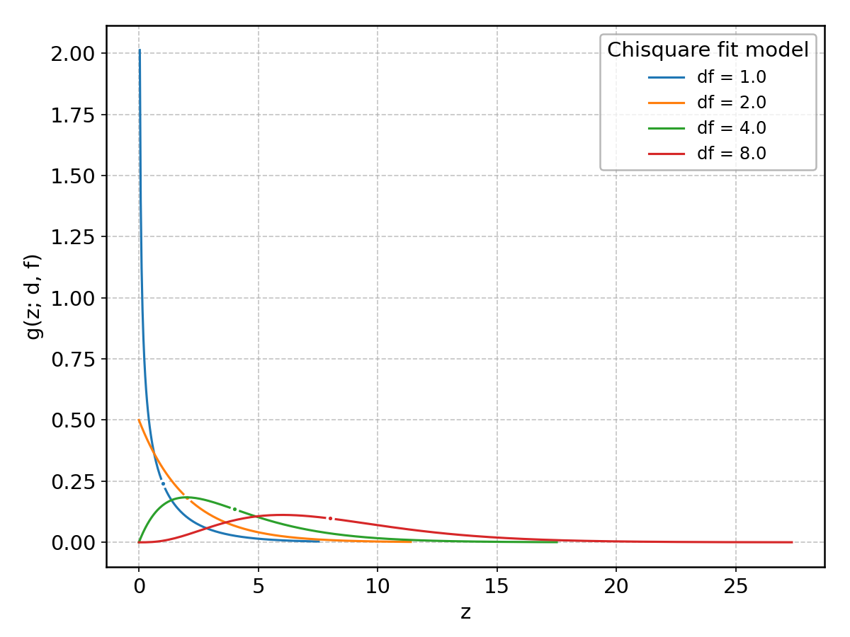
Chisquare

Wrapped from scipy.stats.chi2; support: \(z > 0\) shape parameter(s): \(\text{df} > 0\).

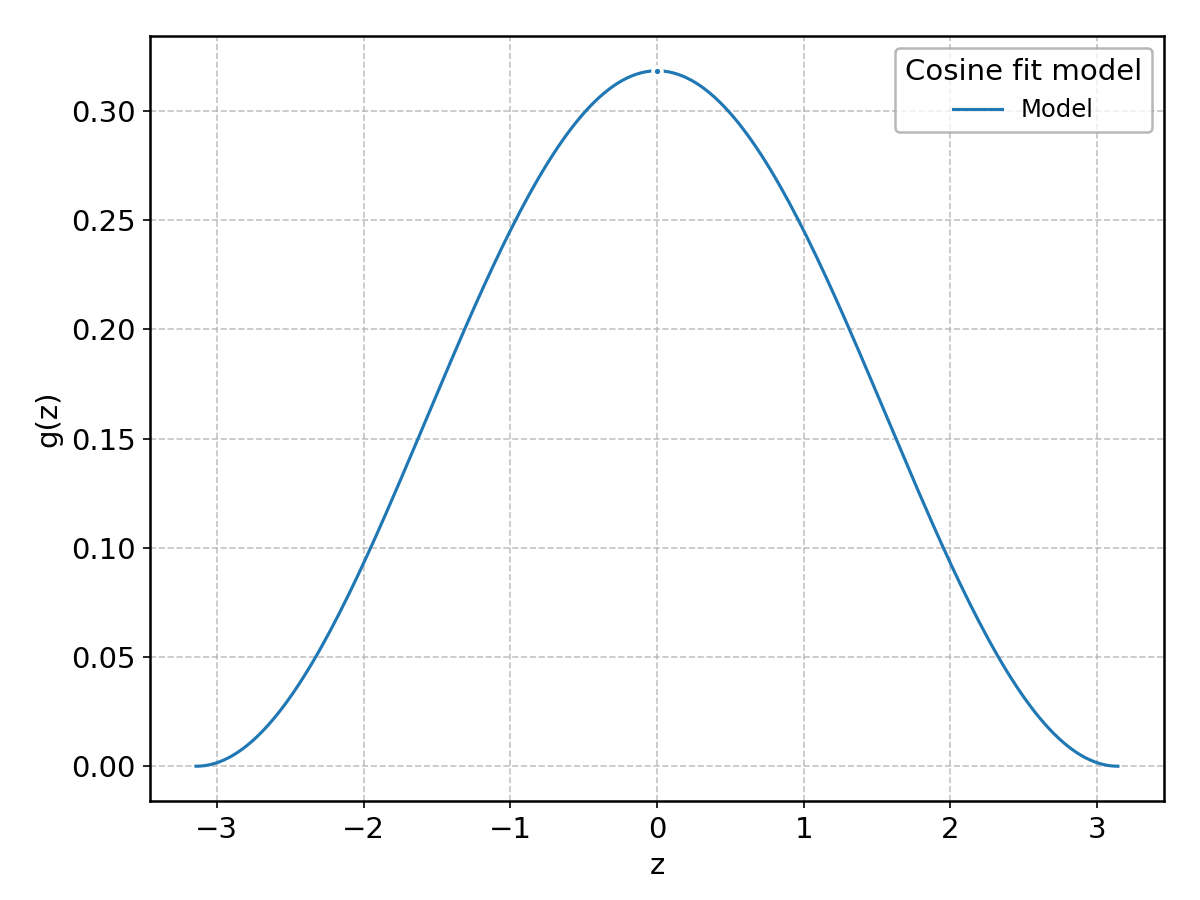
Cosine

Wrapped from scipy.stats.cosine; support: \(-\pi \le z \le \pi\).

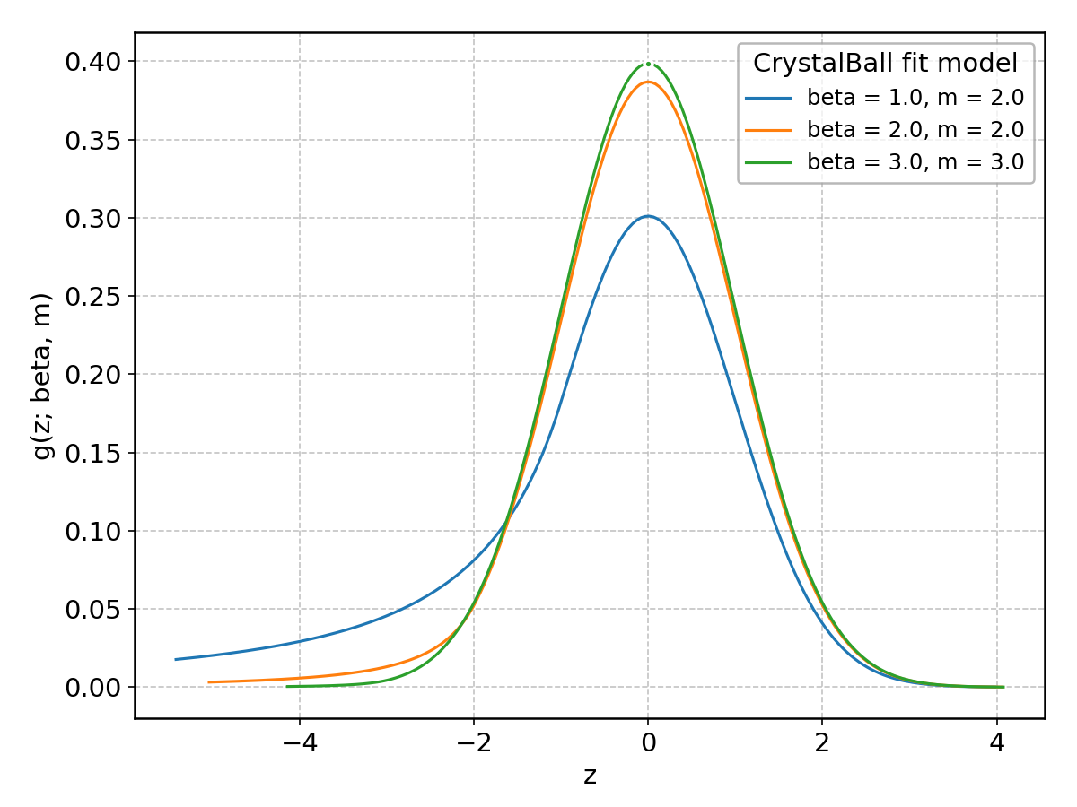
CrystalBall

Wrapped from scipy.stats.crystalball; support: \(-\infty < z < \infty\); shape parameter(s): \(m > 1\), \(\beta > 0\).

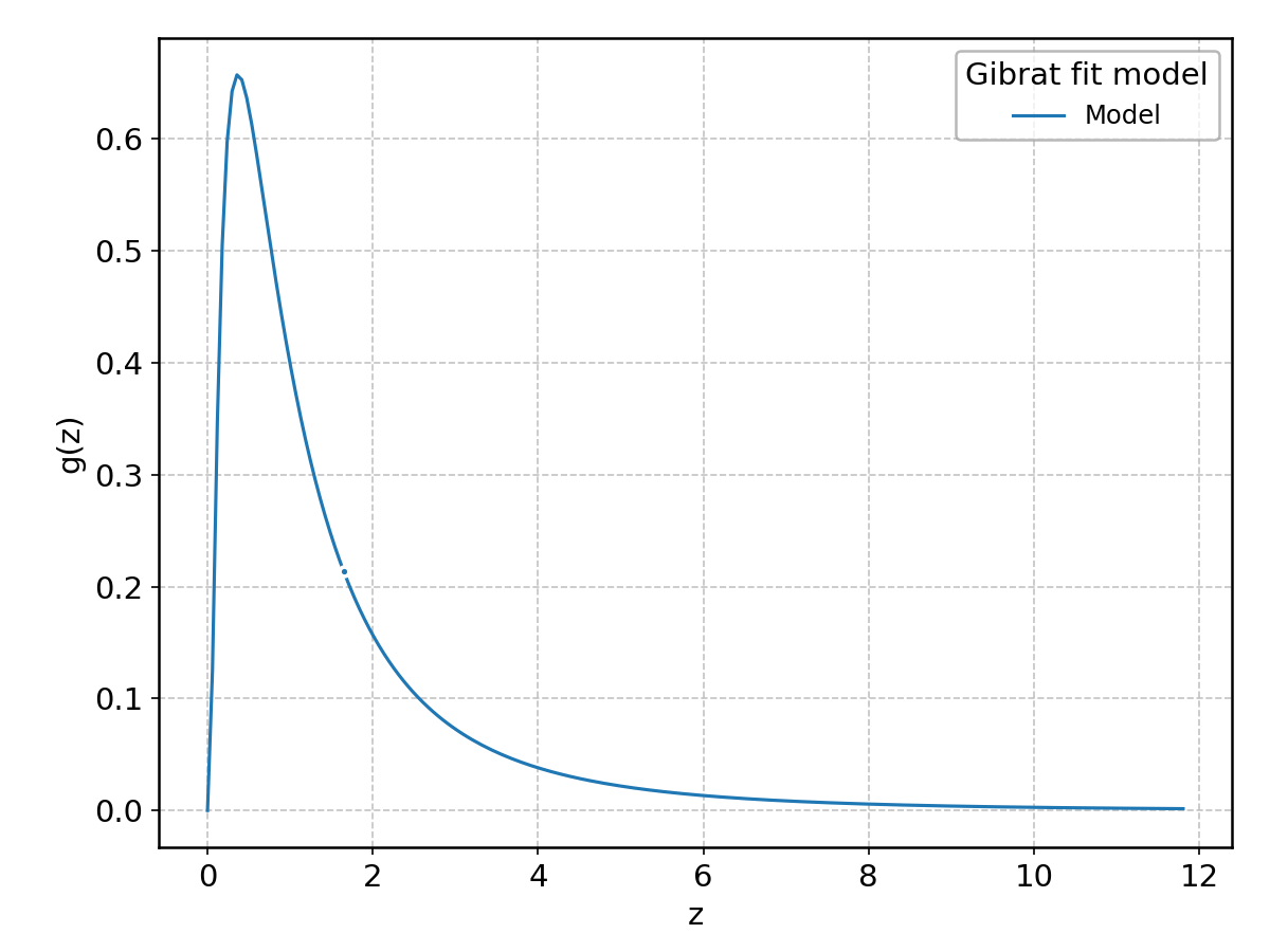
Gibrat

Wrapped from scipy.stats.gibrat; support: \(z > 0\).

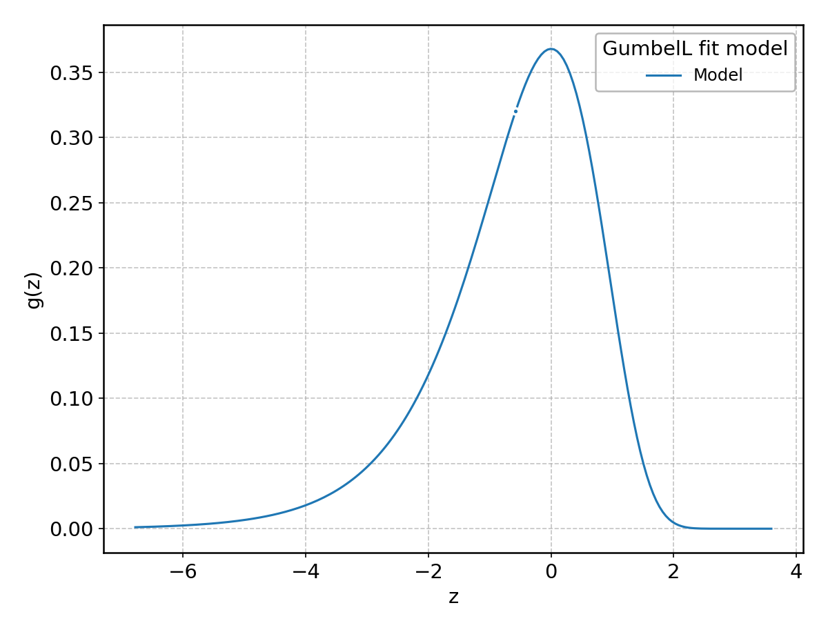
GumbelL

Wrapped from scipy.stats.gumbel_l; support: \(-\infty < z < \infty\).

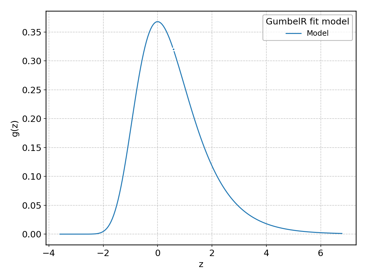
GumbelR

Wrapped from scipy.stats.gumbel_r; support: \(-\infty < z < \infty\).

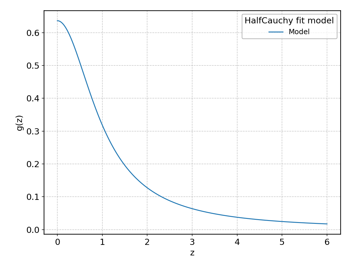
HalfCauchy

Wrapped from scipy.stats.halfcauchy; support: \(z > 0\).

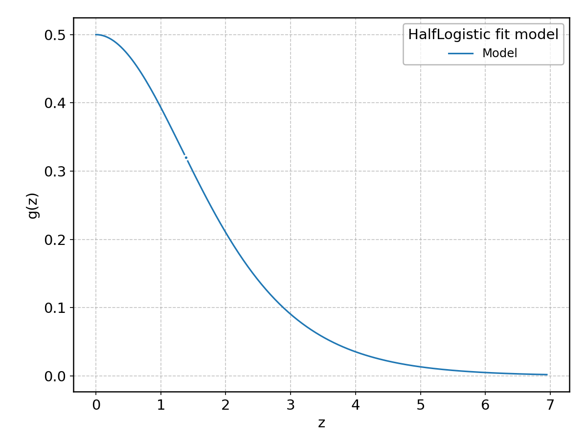
HalfLogistic

Wrapped from scipy.stats.halflogistic; support: \(z > 0\).

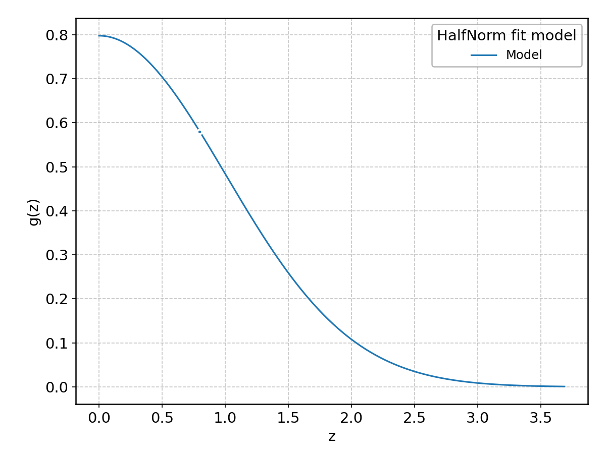
HalfNorm

Wrapped from scipy.stats.halfnorm; support: \(z > 0\).

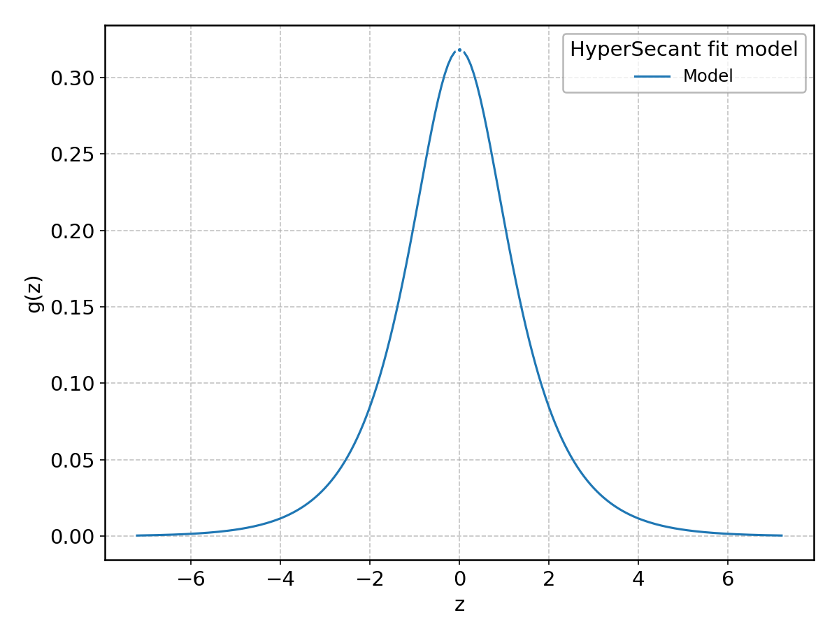
HyperSecant

Wrapped from scipy.stats.hypsecant; support: \(-\infty < z < \infty\).

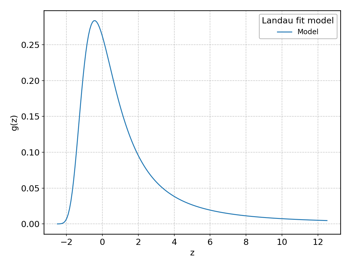
Landau

Wrapped from scipy.stats.landau; support: \(-\infty < z < \infty\).

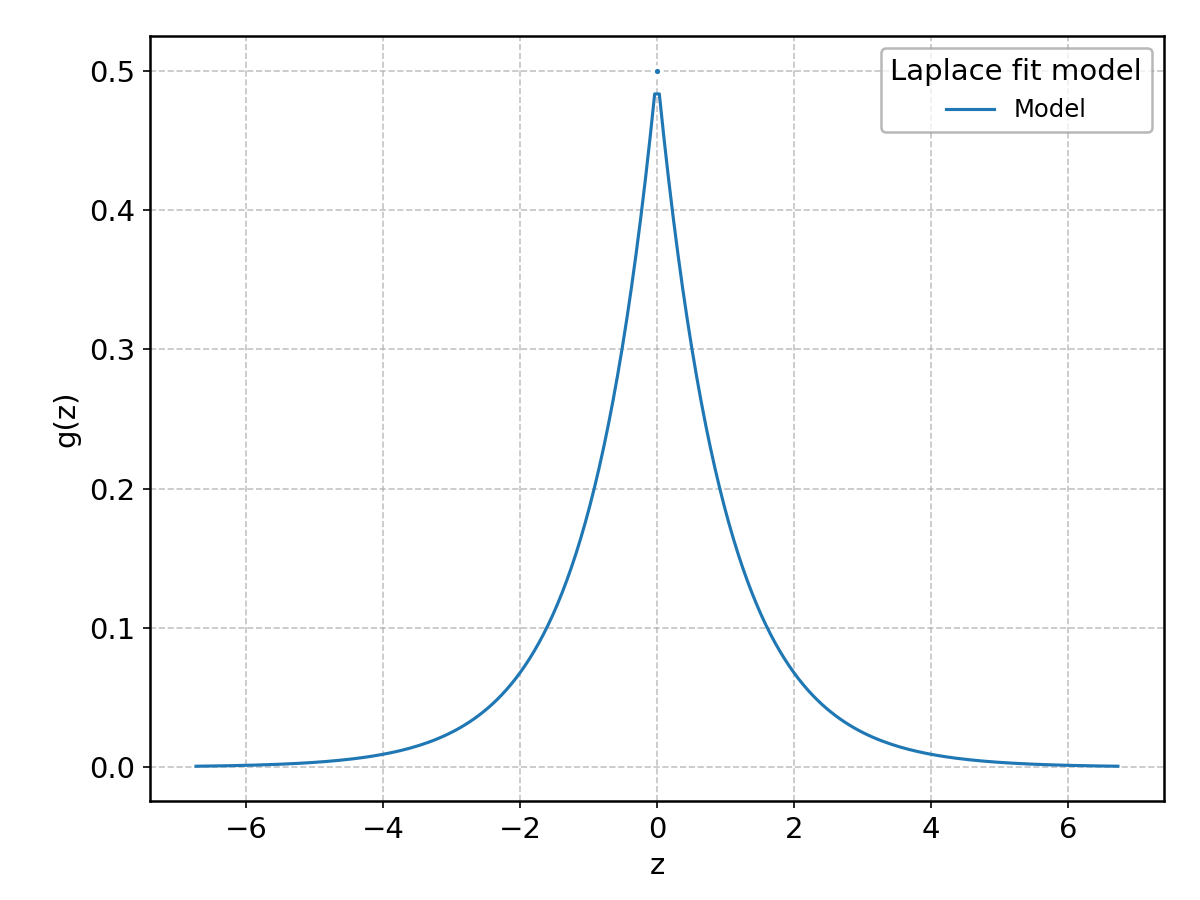
Laplace

Wrapped from scipy.stats.laplace; support: \(-\infty < z < \infty\).

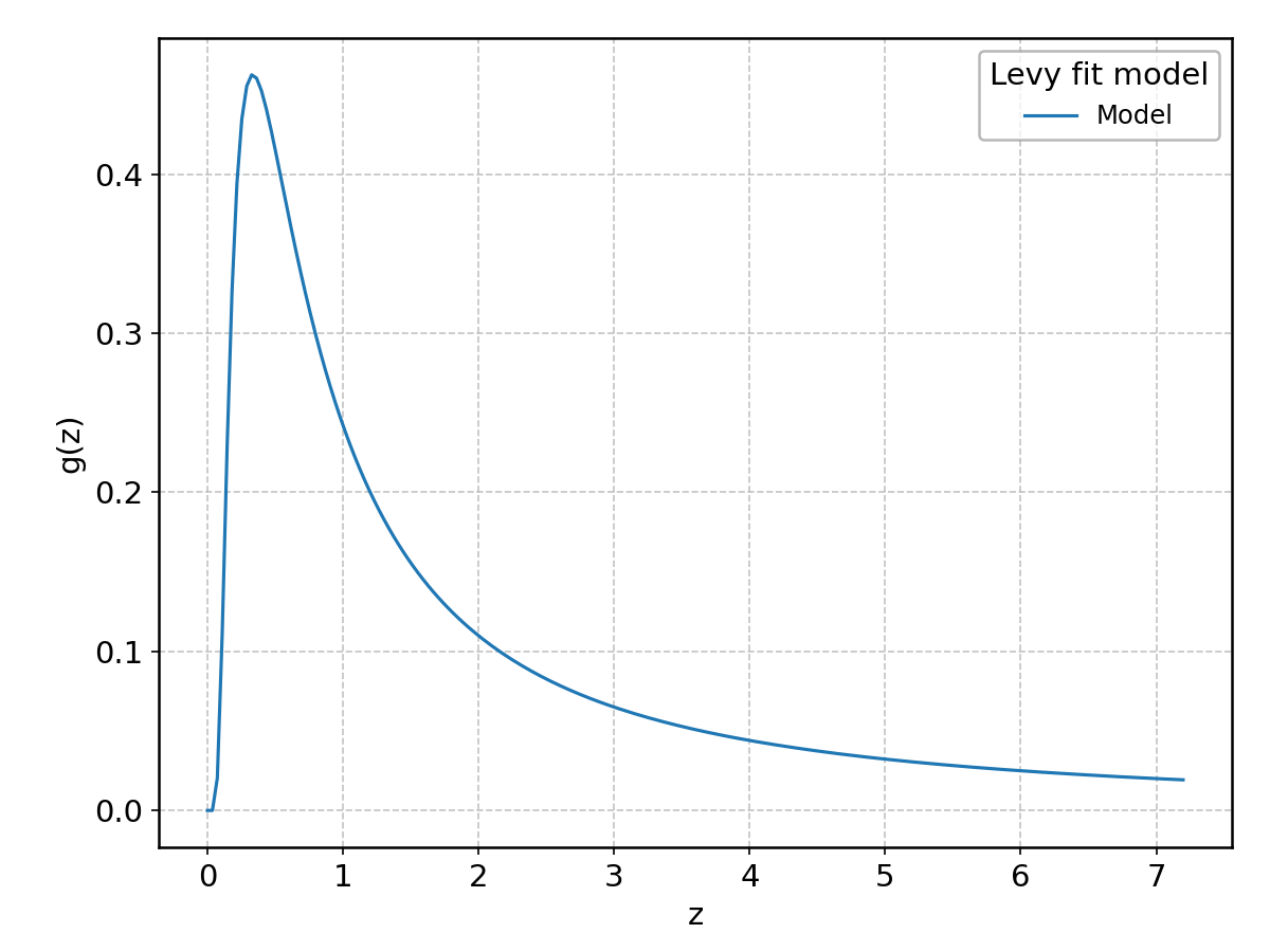
Levy

Wrapped from scipy.stats.levy; support: \(-\infty < z < \infty\).

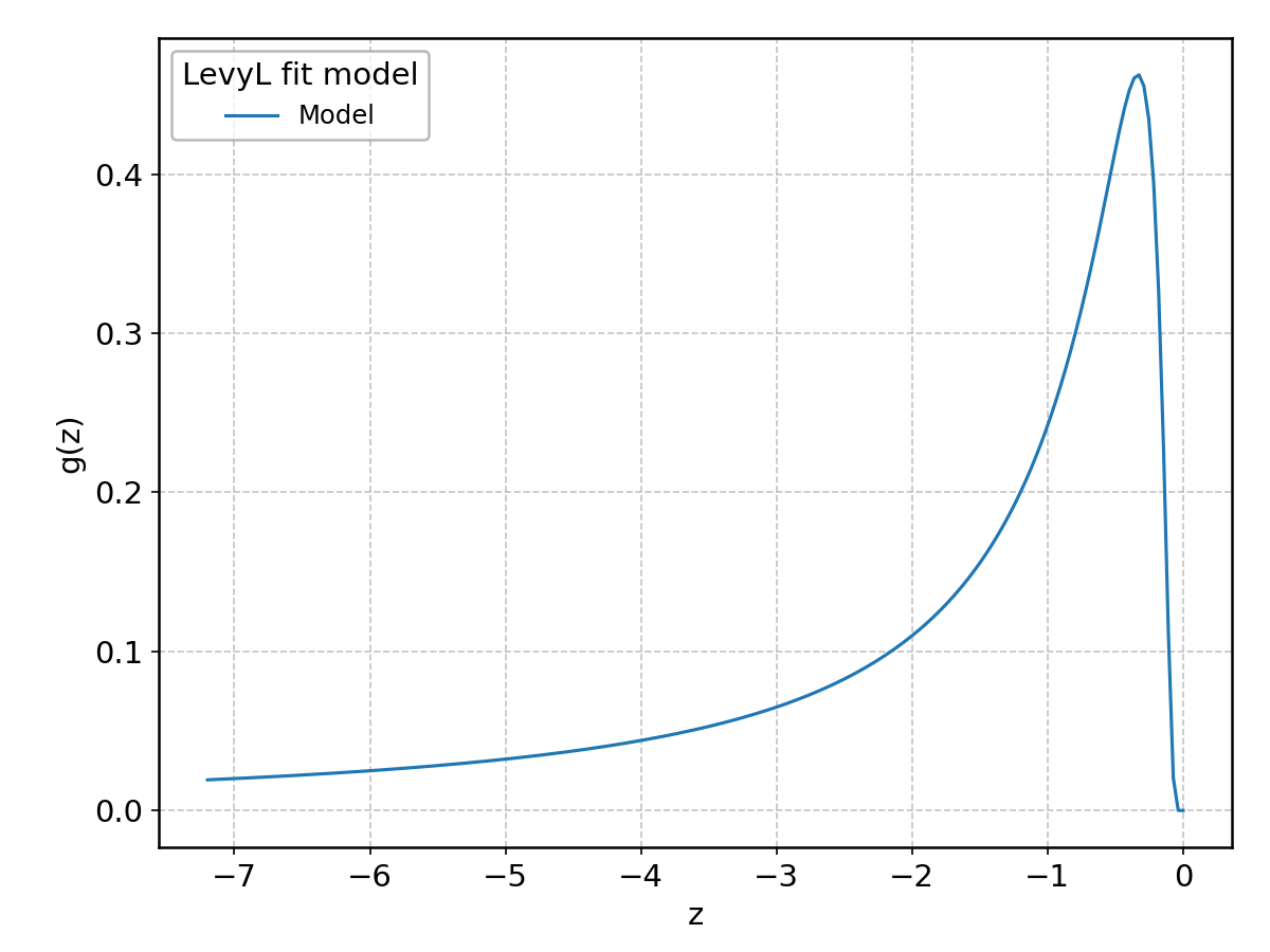
LevyL

Wrapped from scipy.stats.levy_l; support: \(-\infty < z < \infty\).

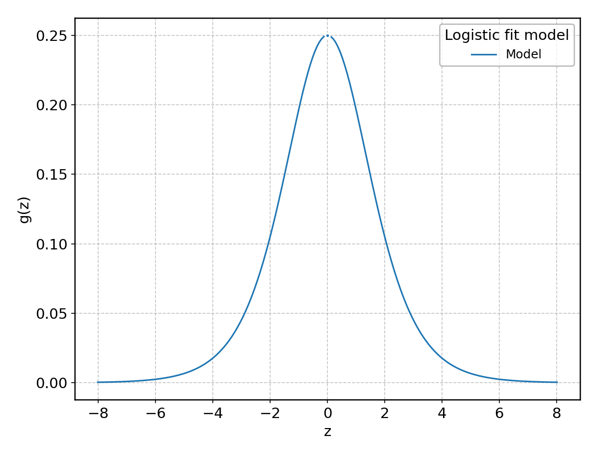
Logistic

Wrapped from scipy.stats.logistic; support: \(-\infty < z < \infty\).

LogNormal

Wrapped from scipy.stats.lognorm; support: \(z > 0\); shape parameter(s): \(s > 0\).

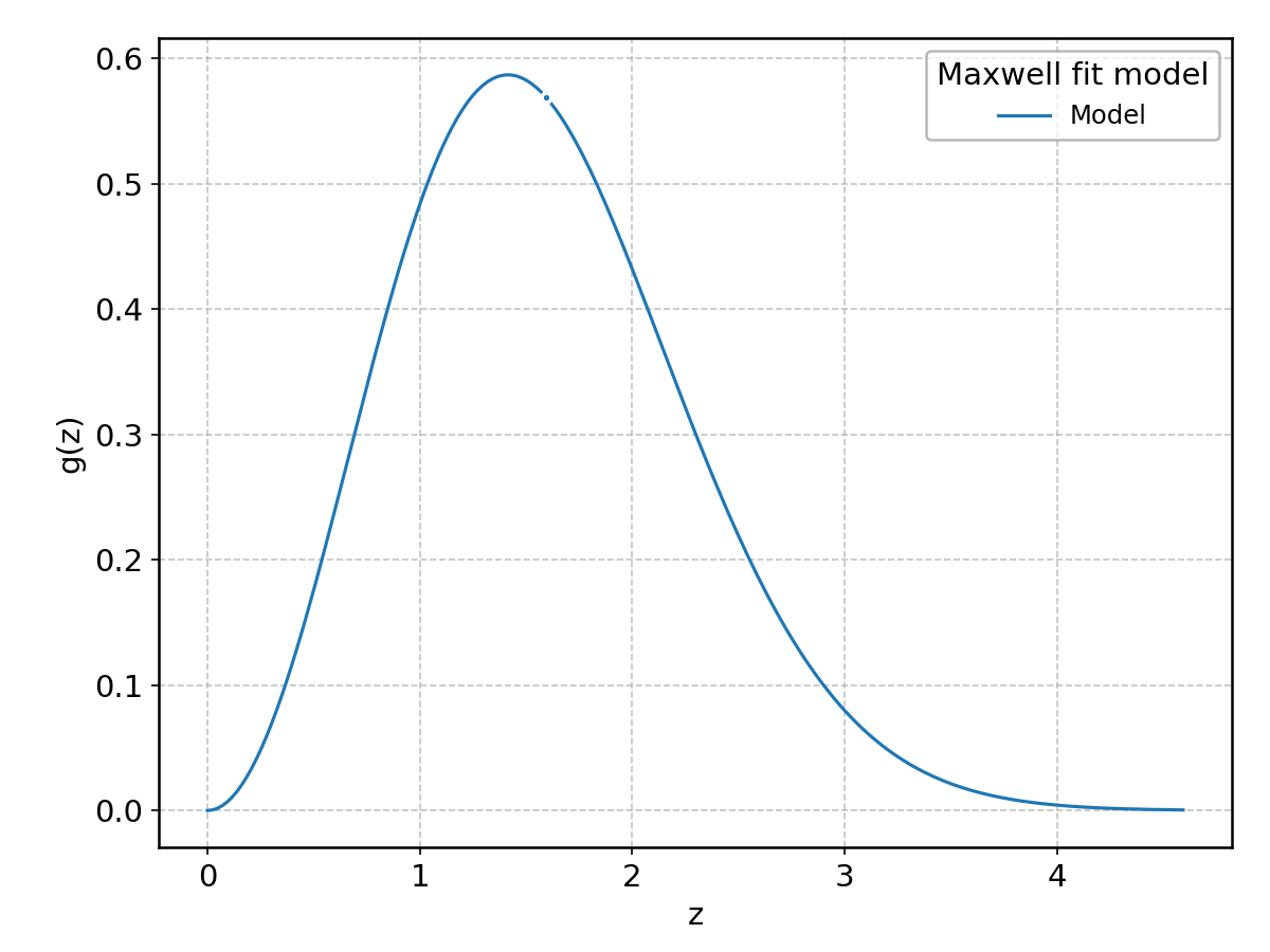
Maxwell

Wrapped from scipy.stats.maxwell; support: \(0 < z < \infty\).

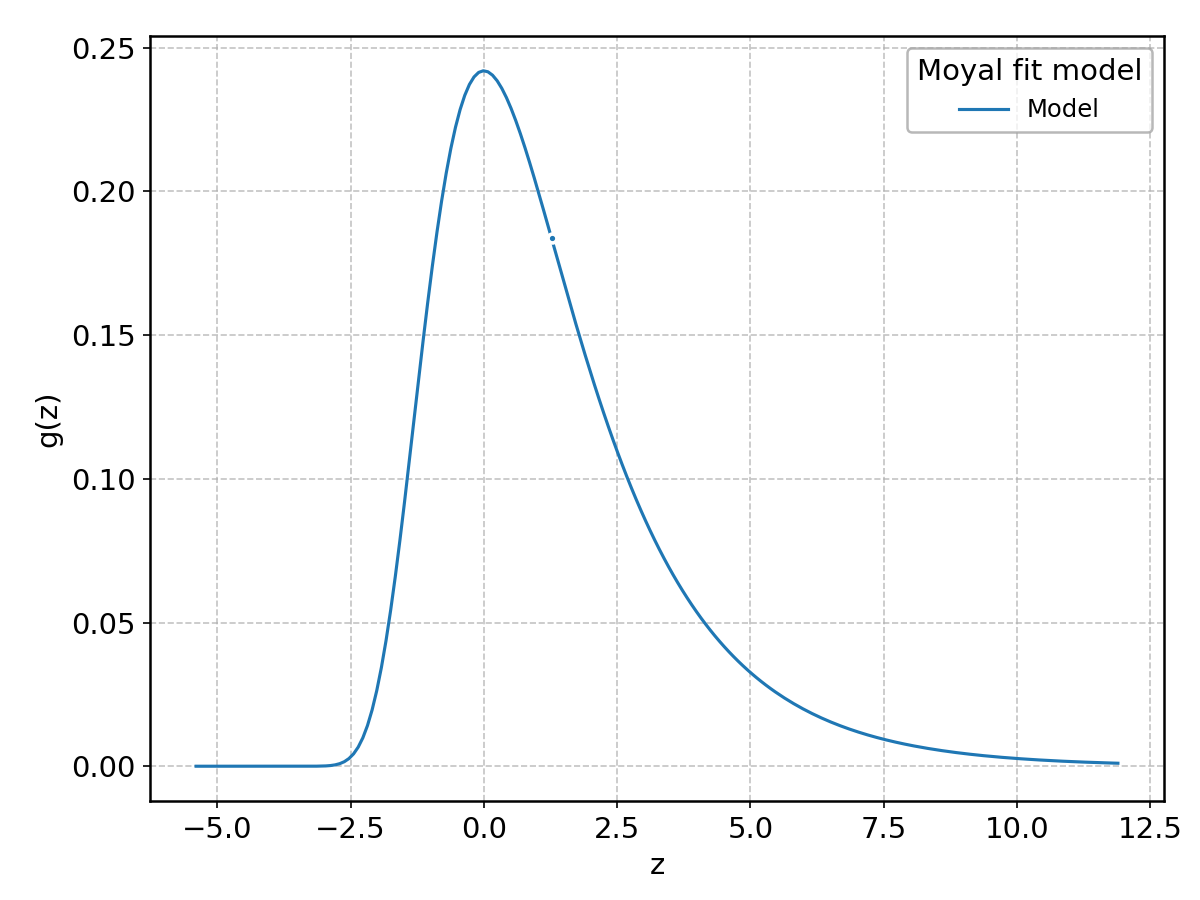
Moyal

Wrapped from scipy.stats.moyal; support: \(-\infty < z < \infty\).

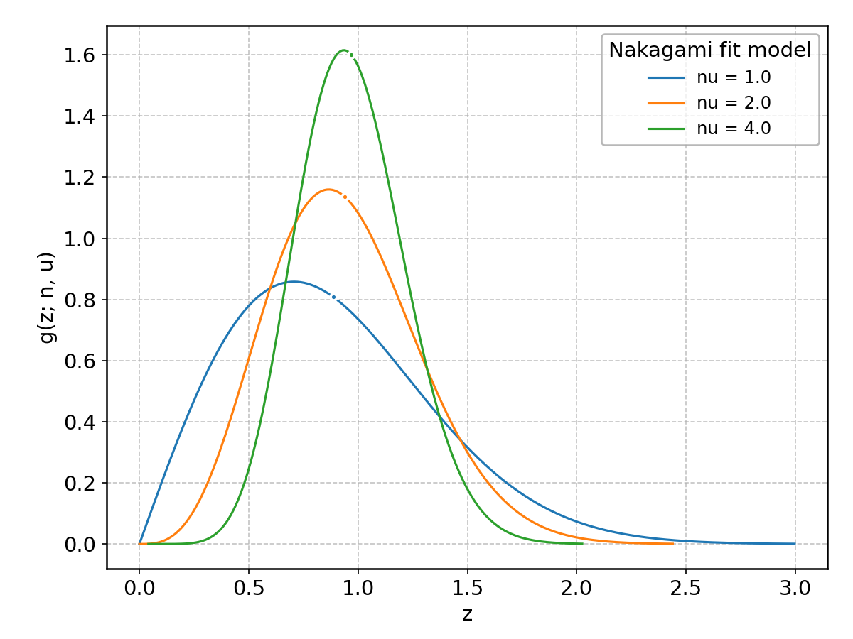
Nakagami

Wrapped from scipy.stats.nakagami; support: \(0 < z < \infty\).

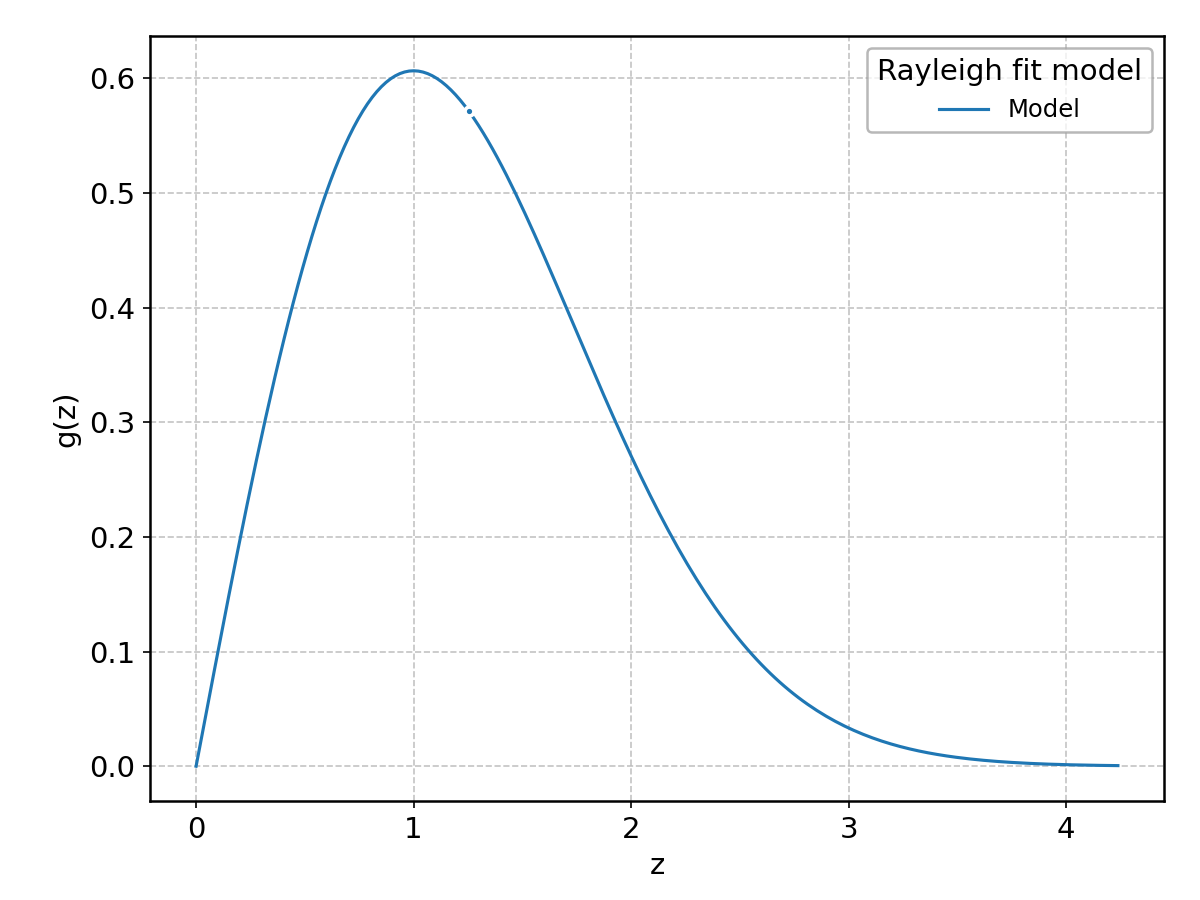
Rayleigh

Wrapped from scipy.stats.rayleigh; support: \(0 < z < \infty\).

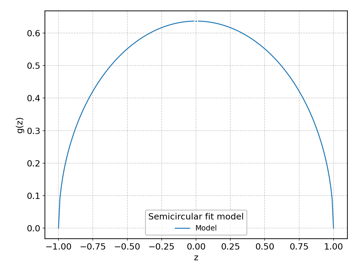
Semicircular

Wrapped from scipy.stats.semicircular; support: \(-\infty < z < \infty\).

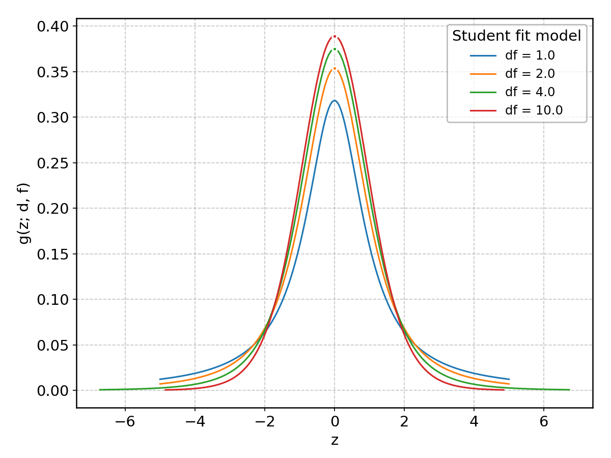
Student

Wrapped from scipy.stats.t; support: \(-\infty < z < \infty\).

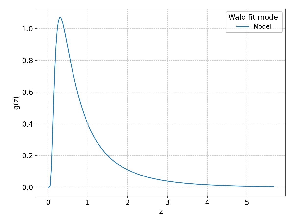
Wald

Wrapped from scipy.stats.wald; support: \(0 < z < \infty\).

Module documentation

Built in models.

class aptapy.models.Constant(label: str = None, xlabel: str = None, ylabel: str = None)

Constant model.

value = FitParameter(value=1.0, _name=None, error=None, _frozen=False, minimum=-inf, maximum=inf)

static evaluate(x: float | ndarray, value: float) → float | ndarray

Evaluate the model at a given set of parameter values.

Arguments

xarray_like

The value(s) of the independent variable.

parameter_valuessequence of float

The value of the model parameters.

Returns

yarray_like

The value(s) of the model at the given value(s) of the independent variable for a given set of parameter values.

init_parameters(xdata: float | ndarray, ydata: float | ndarray, sigma: float | ndarray = 1.0) → None

Overloaded method.

This is simply using the weighted average of the y data, using the inverse of the squares of the errors as weights.

Note

This should provide the exact result in most cases, but, in the spirit of providing a common interface across all models, we are not overloading the fit() method. (Everything will continue working as expected, e.g., when one uses bounds on parameters.)

primitive(x: float | ndarray) → float | ndarray

_abc_impl = <_abc._abc_data object>

class aptapy.models.Line(label: str = None, xlabel: str = None, ylabel: str = None)

Linear model.

slope = FitParameter(value=1.0, _name=None, error=None, _frozen=False, minimum=-inf, maximum=inf)

intercept = FitParameter(value=0.0, _name=None, error=None, _frozen=False, minimum=-inf, maximum=inf)

static evaluate(x: float | ndarray, slope: float, intercept: float) → float | ndarray

Evaluate the model at a given set of parameter values.

Arguments

xarray_like

The value(s) of the independent variable.

parameter_valuessequence of float

The value of the model parameters.

Returns

yarray_like

The value(s) of the model at the given value(s) of the independent variable for a given set of parameter values.

init_parameters(xdata: float | ndarray, ydata: float | ndarray, sigma: float | ndarray = 1.0) → None

Overloaded method.

This is simply using a weighted linear regression.

Note

This should provide the exact result in most cases, but, in the spirit of providing a common interface across all models, we are not overloading the fit() method. (Everything will continue working as expected, e.g., when one uses bounds on parameters.)

primitive(x: float | ndarray) → float | ndarray

_abc_impl = <_abc._abc_data object>

class aptapy.models.Polynomial(degree: int, label: str = None, xlabel: str = None, ylabel: str = None)

Generic polynomial model.

Note that this is a convenience class to be used when one needs polynomials of arbitrary degree. For common low-order polynomials, consider using the dedicated classes (e.g., Line, Quadratic, etc.), which provide better initial parameter estimation.

Arguments

degreeint

The degree of the polynomial.

labelstr, optional

The model label.

xlabelstr, optional

The label for the x axis.

ylabelstr, optional

The label for the y axis.

static evaluate(x: float | ndarray, *coefficients: float) → float | ndarray

Evaluate the model at a given set of parameter values.

Arguments

xarray_like

The value(s) of the independent variable.

parameter_valuessequence of float

The value of the model parameters.

Returns

yarray_like

The value(s) of the model at the given value(s) of the independent variable for a given set of parameter values.

init_parameters(xdata: float | ndarray, ydata: float | ndarray, sigma: float | ndarray = 1.0) → None

Overloaded method.

This is using a weighted linear regression.

Note

This should provide the exact result in most cases, but, in the spirit of providing a common interface across all models, we are not overloading the fit() method. (Everything will continue working as expected, e.g., when one uses bounds on parameters.)

static primitive(x: float | ndarray, *coefficients: float) → float | ndarray

_abc_impl = <_abc._abc_data object>

class aptapy.models.Quadratic(label: str = None, xlabel: str = None, ylabel: str = None)

Quadratic model.

This is just a convenience subclass of the generic Polynomial model with degree fixed to 2.

_abc_impl = <_abc._abc_data object>

class aptapy.models.Cubic(label: str = None, xlabel: str = None, ylabel: str = None)

Cubic model.

This is just a convenience subclass of the generic Polynomial model with degree fixed to 3.

_abc_impl = <_abc._abc_data object>

class aptapy.models.PowerLaw(pivot: float = 1.0, label: str = None, xlabel: str = None, ylabel: str = None)

Power-law model.

Arguments

pivotfloat, optional

The pivot point of the power-law (default 1.).

labelstr, optional

The model label.

xlabelstr, optional

The label for the x axis.

ylabelstr, optional

The label for the y axis.

prefactor = FitParameter(value=1.0, _name=None, error=None, _frozen=False, minimum=-inf, maximum=inf)

index = FitParameter(value=-2.0, _name=None, error=None, _frozen=False, minimum=-inf, maximum=inf)

evaluate(x: float | ndarray, prefactor: float, index: float) → float | ndarray

Evaluate the model at a given set of parameter values.

Arguments

xarray_like

The value(s) of the independent variable.

parameter_valuessequence of float

The value of the model parameters.

Returns

yarray_like

The value(s) of the model at the given value(s) of the independent variable for a given set of parameter values.

init_parameters(xdata: float | ndarray, ydata: float | ndarray, sigma: float | ndarray = 1.0) → None

Overloaded method.

This is using a weighted linear regression in log-log space. Note this is not an exact solution in the original space, for which a numerical optimization using non-linear least squares would be needed.

primitive(x: float | ndarray) → float | ndarray

Overloaded method.

default_plotting_range() → Tuple[float, float]

Overloaded method.

We might be smarter here, but for now we just return a fixed range that is not bogus when the index is negative, which should cover the most common use cases.

plot(axes: Axes = None, fit_output: bool = False, **kwargs) → None

Overloaded method.

In addition to the base class implementation, this also sets log scales on both axes.

_abc_impl = <_abc._abc_data object>

class aptapy.models.Exponential(location: float = 0.0, label: str = None, xlabel: str = None, ylabel: str = None)

Exponential model.

Note this is an example of a model with a state, i.e., one where evaluate() is not a static method, as we have a location attribute that needs to be taken into account. This is done in the spirit of facilitating fits where the exponential decay starts at a non-zero x value.

(One might argue that location should be a fit parameter as well, but that would be degenerate with the scale parameter, and it would have to be fixed in most cases anyway, so a simple attribute seems more appropriate here.)

Arguments

locationfloat, optional

The location of the exponential decay (default 0.).

labelstr, optional

The model label.

xlabelstr, optional

The label for the x axis.

ylabelstr, optional

The label for the y axis.

prefactor = FitParameter(value=1.0, _name=None, error=None, _frozen=False, minimum=-inf, maximum=inf)

scale = FitParameter(value=1.0, _name=None, error=None, _frozen=False, minimum=-inf, maximum=inf)

evaluate(x: float | ndarray, prefactor: float, scale: float) → float | ndarray

Evaluate the model at a given set of parameter values.

Arguments

xarray_like

The value(s) of the independent variable.

parameter_valuessequence of float

The value of the model parameters.

Returns

yarray_like

The value(s) of the model at the given value(s) of the independent variable for a given set of parameter values.

init_parameters(xdata: float | ndarray, ydata: float | ndarray, sigma: float | ndarray = 1.0) → None

Overloaded method.

This is using a weighted linear regression in lin-log space. Note this is not an exact solution in the original space, for which a numerical optimization using non-linear least squares would be needed.

primitive(x: float | ndarray) → float | ndarray

default_plotting_range(scale_factor: int = 5) → Tuple[float, float]

Overloaded method.

_abc_impl = <_abc._abc_data object>

class aptapy.models.ExponentialComplement(location: float = 0.0, label: str = None, xlabel: str = None, ylabel: str = None)

Exponential complement model.

evaluate(x: float | ndarray, prefactor: float, scale: float) → float | ndarray

Evaluate the model at a given set of parameter values.

Arguments

xarray_like

The value(s) of the independent variable.

parameter_valuessequence of float

The value of the model parameters.

Returns

yarray_like

The value(s) of the model at the given value(s) of the independent variable for a given set of parameter values.

init_parameters(xdata: float | ndarray, ydata: float | ndarray, sigma: float | ndarray = 1.0) → None

Overloaded method.

Note we just pretend that the maximum of the y values is a reasonable estimate of the prefactor, and go back to the plain exponential case via the transformation ydata -> prefactor - ydata.

_abc_impl = <_abc._abc_data object>

class aptapy.models.StretchedExponential(location: float = 0.0, label: str = None, xlabel: str = None, ylabel: str = None)

Stretched exponential model.

stretch = FitParameter(value=1.0, _name=None, error=None, _frozen=False, minimum=0.0, maximum=inf)

evaluate(x: float | ndarray, prefactor: float, scale: float, stretch: float) → float | ndarray

Evaluate the model at a given set of parameter values.

Arguments

xarray_like

The value(s) of the independent variable.

parameter_valuessequence of float

The value of the model parameters.

Returns

yarray_like

The value(s) of the model at the given value(s) of the independent variable for a given set of parameter values.

init_parameters(xdata: float | ndarray, ydata: float | ndarray, sigma: float | ndarray = 1.0)

Overloaded method.

Note this a little bit flaky, in that we pretend that the data are well approximated by a plain exponential, and do not even try at estimating the stretch factor. When the latter is significantly different from 1 this will not be very accurate, but hopefully good enough to get the fit started.

default_plotting_range(scale_factor: int = 5) → Tuple[float, float]

Overloaded method.

_abc_impl = <_abc._abc_data object>

class aptapy.models.StretchedExponentialComplement(location: float = 0.0, label: str = None, xlabel: str = None, ylabel: str = None)

Stretched exponential complement model.

evaluate(x: float | ndarray, prefactor: float, scale: float, stretch: float) → float | ndarray

Evaluate the model at a given set of parameter values.

Arguments

xarray_like

The value(s) of the independent variable.

parameter_valuessequence of float

The value of the model parameters.

Returns

yarray_like

The value(s) of the model at the given value(s) of the independent variable for a given set of parameter values.

init_parameters(xdata: float | ndarray, ydata: float | ndarray, sigma: float | ndarray = 1.0) → None

Overloaded method.

See the comment in the corresponding docstrings of the ExponentialComplement class.

_abc_impl = <_abc._abc_data object>

class aptapy.models.Gaussian(label: str = None, xlabel: str = None, ylabel: str = None)

This is a re-implementation from scratch of the normal distribution, which is also available as a wrapper around scipy.stats.norm as Normal.

The main reason for this is to be able to call the underlying parameters with more familiar names (mu, sigma, rather than loc, scale), as well as providing additional convenience methods such the iterative fitting around the peak.

amplitude = FitParameter(value=1.0, _name=None, error=None, _frozen=False, minimum=-inf, maximum=inf)

mu = FitParameter(value=0.0, _name=None, error=None, _frozen=False, minimum=-inf, maximum=inf)

sigma = FitParameter(value=1.0, _name=None, error=None, _frozen=False, minimum=0.0, maximum=inf)

static evaluate(x, amplitude, mu, sigma, *args)

Evaluate the model at a given set of parameter values.

Arguments

xarray_like

The value(s) of the independent variable.

parameter_valuessequence of float

The value of the model parameters.

Returns

yarray_like

The value(s) of the model at the given value(s) of the independent variable for a given set of parameter values.

static primitive(x, amplitude, mu, sigma, *args)

median()

mean()

std()

fwhm()

Calculate the FWHM.

rvs(size: int = 1, random_state=None)

Generate random variates from the underlying distribution at the current parameter values.

Arguments

sizeint, optional

The number of random variates to generate (default 1).

random_stateint or np.random.Generator, optional

The random seed or generator to use (default None).

init_parameters(xdata: float | ndarray, ydata: float | ndarray, sigma: float | ndarray = 1.0) → None

Overloaded method.

fit_iterative(xdata: float | ndarray | Histogram1d, ydata: float | ndarray = None, *, p0: float | ndarray = None, sigma: float | ndarray = None, num_sigma_left: float = 2.0, num_sigma_right: float = 2.0, num_iterations: int = 2, **kwargs) → FitStatus

Fit the core of Gaussian data within a given number of sigma around the peak.

This function performs a first round of fit to the data (either a histogram or scatter plot data) and then repeats the fit iteratively, limiting the fit range to a specified interval defined in terms of deviations (in sigma) around the peak.

Arguments

xdataarray_like or Histogram1d

The data (scatter plot x values) or histogram to fit.

ydataarray_like, optional

The y data to fit (if xdata is not a Histogram1d).

p0array_like, optional

The initial values for the fit parameters.

sigmaarray_like, optional

The uncertainties on the y data.

num_sigma_leftfloat

The number of sigma on the left of the peak to be used to define the fitting range.

num_sigma_rightfloat

The number of sigma on the right of the peak to be used to define the fitting range.

num_iterationsint

The number of iterations of the fit.

kwargsdict, optional

Additional keyword arguments passed to fit().

Returns

FitStatus

The results of the fit.

default_plotting_range() → Tuple[float, float]

Overloaded method.

plot(axes: Axes = None, fit_output: bool = False, plot_mean: bool = True, **kwargs) → None

Plot the model.

Note this is reimplemented from scratch to allow overplotting the mean of the distribution.

Arguments

axesmatplotlib.axes.Axes, optional

The axes to plot on (default: current axes).

fit_outputbool, optional

Whether to include the fit output in the legend (default: False).

plot_meanbool, optional

Whether to overplot the mean of the distribution (default: True).

kwargsdict, optional

Additional keyword arguments passed to plt.plot().

_abc_impl = <_abc._abc_data object>

class aptapy.models.Fe55Forest(label: str = None, xlabel: str = None, ylabel: str = None)

Model representing the Kα and Kβ emission lines produced in the decay of 55Fe. The energy values are computed as the intensity-weighted mean of all possible emission lines contributing to each feature.

The energy data are retrieved from the X-ray database at https://xraydb.seescience.org/

TABULATED_KB_INTENSITY = 0.12445

init_parameters(xdata: float | ndarray, ydata: float | ndarray, sigma: float | ndarray = 1.0) → None

Overloaded method.

_abc_impl = <_abc._abc_data object>

amplitude = FitParameter(value=1.0, _name=None, error=None, _frozen=False, minimum=0.0, maximum=inf)

energies = (5.896, 6.492)

energy_scale = FitParameter(value=1.0, _name=None, error=None, _frozen=False, minimum=0.0, maximum=inf)

intensity1 = FitParameter(value=0.5, _name=None, error=None, _frozen=False, minimum=0.0, maximum=1.0)

sigma = FitParameter(value=1.0, _name=None, error=None, _frozen=False, minimum=0.0, maximum=inf)

class aptapy.models.Probit(label: str = None, xlabel: str = None, ylabel: str = None)

Custom implementation of the probit model, i.e., the percent-point function of a gaussian distribution.

offset = FitParameter(value=0.0, _name=None, error=None, _frozen=False, minimum=-inf, maximum=inf)

sigma = FitParameter(value=1.0, _name=None, error=None, _frozen=False, minimum=0.0, maximum=inf)

static evaluate(x: float | ndarray, offset: float, sigma: float) → float | ndarray

Evaluate the model at a given set of parameter values.

Arguments

xarray_like

The value(s) of the independent variable.

parameter_valuessequence of float

The value of the model parameters.

Returns

yarray_like

The value(s) of the model at the given value(s) of the independent variable for a given set of parameter values.

init_parameters(xdata: float | ndarray, ydata: float | ndarray, sigma: float | ndarray = 1.0) → None

Overloaded method.

static default_plotting_range() → Tuple[float, float]

Overloaded method.

Since the probit function diverges at 0 and 1, we limit the plotting range to a reasonable interval.

_abc_impl = <_abc._abc_data object>

class aptapy.models.ErfSigmoid(label: str = None, xlabel: str = None, ylabel: str = None)

Error function model.

static shape(z)

Abstract method for the normalized shape of the sigmoid model. Subclasses must implement this method.

Arguments

zarray_like

The normalized independent variable.

parameter_valuesfloat

Additional shape parameters for the sigmoid.

Returns

array_like

The value of the sigmoid shape function at z.

_abc_impl = <_abc._abc_data object>

class aptapy.models.LogisticSigmoid(label: str = None, xlabel: str = None, ylabel: str = None)

Logistic function model.

static shape(z)

Abstract method for the normalized shape of the sigmoid model. Subclasses must implement this method.

Arguments

zarray_like

The normalized independent variable.

parameter_valuesfloat

Additional shape parameters for the sigmoid.

Returns

array_like

The value of the sigmoid shape function at z.

_abc_impl = <_abc._abc_data object>

class aptapy.models.Arctangent(label: str = None, xlabel: str = None, ylabel: str = None)

Arctangent function model.

static shape(z)

Abstract method for the normalized shape of the sigmoid model. Subclasses must implement this method.

Arguments

zarray_like

The normalized independent variable.

parameter_valuesfloat

Additional shape parameters for the sigmoid.

Returns

array_like

The value of the sigmoid shape function at z.

_abc_impl = <_abc._abc_data object>

class aptapy.models.HyperbolicTangent(label: str = None, xlabel: str = None, ylabel: str = None)

Hyperbolic tangent function model.

static shape(z)

Abstract method for the normalized shape of the sigmoid model. Subclasses must implement this method.

Arguments

zarray_like

The normalized independent variable.

parameter_valuesfloat

Additional shape parameters for the sigmoid.

Returns

array_like

The value of the sigmoid shape function at z.

_abc_impl = <_abc._abc_data object>

class aptapy.models.Alpha(label: str = None, xlabel: str = None, ylabel: str = None)

_abc_impl = <_abc._abc_data object>

_rv = <scipy.stats._continuous_distns.alpha_gen object>

a = FitParameter(value=1.0, _name=None, error=None, _frozen=False, minimum=0.0, maximum=inf)

class aptapy.models.Anglit(label: str = None, xlabel: str = None, ylabel: str = None)

_abc_impl = <_abc._abc_data object>

_rv = <scipy.stats._continuous_distns.anglit_gen object>

class aptapy.models.Arcsine(label: str = None, xlabel: str = None, ylabel: str = None)

_abc_impl = <_abc._abc_data object>

_rv = <scipy.stats._continuous_distns.arcsine_gen object>

class aptapy.models.Argus(label: str = None, xlabel: str = None, ylabel: str = None)

_abc_impl = <_abc._abc_data object>

_rv = <scipy.stats._continuous_distns.argus_gen object>

chi = FitParameter(value=1.0, _name=None, error=None, _frozen=False, minimum=0.0, maximum=inf)

class aptapy.models.Beta(label: str = None, xlabel: str = None, ylabel: str = None)

_abc_impl = <_abc._abc_data object>

_rv = <scipy.stats._continuous_distns.beta_gen object>

a = FitParameter(value=1.0, _name=None, error=None, _frozen=False, minimum=0.0, maximum=inf)

b = FitParameter(value=1.0, _name=None, error=None, _frozen=False, minimum=0.0, maximum=inf)

class aptapy.models.BetaPrime(label: str = None, xlabel: str = None, ylabel: str = None)

_abc_impl = <_abc._abc_data object>

_rv = <scipy.stats._continuous_distns.betaprime_gen object>

a = FitParameter(value=1.0, _name=None, error=None, _frozen=False, minimum=0.0, maximum=inf)

b = FitParameter(value=1.0, _name=None, error=None, _frozen=False, minimum=0.0, maximum=inf)

class aptapy.models.Bradford(label: str = None, xlabel: str = None, ylabel: str = None)

_abc_impl = <_abc._abc_data object>

_rv = <scipy.stats._continuous_distns.bradford_gen object>

c = FitParameter(value=1.0, _name=None, error=None, _frozen=False, minimum=0.0, maximum=inf)

class aptapy.models.Burr(label: str = None, xlabel: str = None, ylabel: str = None)

_abc_impl = <_abc._abc_data object>

_rv = <scipy.stats._continuous_distns.burr_gen object>

c = FitParameter(value=1.0, _name=None, error=None, _frozen=False, minimum=0.0, maximum=inf)

d = FitParameter(value=1.0, _name=None, error=None, _frozen=False, minimum=0.0, maximum=inf)

class aptapy.models.Burr12(label: str = None, xlabel: str = None, ylabel: str = None)

_abc_impl = <_abc._abc_data object>

_rv = <scipy.stats._continuous_distns.burr12_gen object>

c = FitParameter(value=1.0, _name=None, error=None, _frozen=False, minimum=0.0, maximum=inf)

d = FitParameter(value=1.0, _name=None, error=None, _frozen=False, minimum=0.0, maximum=inf)

class aptapy.models.Cauchy(label: str = None, xlabel: str = None, ylabel: str = None)

_abc_impl = <_abc._abc_data object>

_rv = <scipy.stats._continuous_distns.cauchy_gen object>

class aptapy.models.Chi(label: str = None, xlabel: str = None, ylabel: str = None)

_abc_impl = <_abc._abc_data object>

_rv = <scipy.stats._continuous_distns.chi_gen object>

df = FitParameter(value=1.0, _name=None, error=None, _frozen=False, minimum=0.0, maximum=inf)

class aptapy.models.Chisquare(label: str = None, xlabel: str = None, ylabel: str = None)

_abc_impl = <_abc._abc_data object>

_rv = <scipy.stats._continuous_distns.chi2_gen object>

df = FitParameter(value=1.0, _name=None, error=None, _frozen=False, minimum=0.0, maximum=inf)

class aptapy.models.Cosine(label: str = None, xlabel: str = None, ylabel: str = None)

_abc_impl = <_abc._abc_data object>

_rv = <scipy.stats._continuous_distns.cosine_gen object>

class aptapy.models.CrystalBall(label: str = None, xlabel: str = None, ylabel: str = None)

_abc_impl = <_abc._abc_data object>

_rv = <scipy.stats._continuous_distns.crystalball_gen object>

beta = FitParameter(value=1.0, _name=None, error=None, _frozen=False, minimum=0.0, maximum=inf)

m = FitParameter(value=2.0, _name=None, error=None, _frozen=False, minimum=1.0, maximum=inf)

class aptapy.models.Gibrat(label: str = None, xlabel: str = None, ylabel: str = None)

_abc_impl = <_abc._abc_data object>

_rv = <scipy.stats._continuous_distns.gibrat_gen object>

class aptapy.models.GumbelL(label: str = None, xlabel: str = None, ylabel: str = None)

_abc_impl = <_abc._abc_data object>

_rv = <scipy.stats._continuous_distns.gumbel_l_gen object>

class aptapy.models.GumbelR(label: str = None, xlabel: str = None, ylabel: str = None)

_abc_impl = <_abc._abc_data object>

_rv = <scipy.stats._continuous_distns.gumbel_r_gen object>

class aptapy.models.HalfCauchy(label: str = None, xlabel: str = None, ylabel: str = None)

_abc_impl = <_abc._abc_data object>

_rv = <scipy.stats._continuous_distns.halfcauchy_gen object>

class aptapy.models.HalfLogistic(label: str = None, xlabel: str = None, ylabel: str = None)

_abc_impl = <_abc._abc_data object>

_rv = <scipy.stats._continuous_distns.halflogistic_gen object>

class aptapy.models.HalfNorm(label: str = None, xlabel: str = None, ylabel: str = None)

_abc_impl = <_abc._abc_data object>

_rv = <scipy.stats._continuous_distns.halfnorm_gen object>

class aptapy.models.HyperSecant(label: str = None, xlabel: str = None, ylabel: str = None)

_abc_impl = <_abc._abc_data object>

_rv = <scipy.stats._continuous_distns.hypsecant_gen object>

class aptapy.models.Landau(label: str = None, xlabel: str = None, ylabel: str = None)

default_plotting_range() → Tuple[float, float]

Overloaded method.

The Landau distribution is peculiar in that it has no definite mean or variance, and its support is unbounded. It is also asymmetric, with a long right tail. Therefore, we resort to a custom function for the plotting range.

_abc_impl = <_abc._abc_data object>

_rv = <scipy.stats._continuous_distns.landau_gen object>

class aptapy.models.Laplace(label: str = None, xlabel: str = None, ylabel: str = None)

_abc_impl = <_abc._abc_data object>

_rv = <scipy.stats._continuous_distns.laplace_gen object>

class aptapy.models.Levy(label: str = None, xlabel: str = None, ylabel: str = None)

_abc_impl = <_abc._abc_data object>

_rv = <scipy.stats._continuous_distns.levy_gen object>

class aptapy.models.LevyL(label: str = None, xlabel: str = None, ylabel: str = None)

_abc_impl = <_abc._abc_data object>

_rv = <scipy.stats._continuous_distns.levy_l_gen object>

class aptapy.models.Logistic(label: str = None, xlabel: str = None, ylabel: str = None)

_abc_impl = <_abc._abc_data object>

_rv = <scipy.stats._continuous_distns.logistic_gen object>

class aptapy.models.LogNormal(label: str = None, xlabel: str = None, ylabel: str = None)

_abc_impl = <_abc._abc_data object>

_rv = <scipy.stats._continuous_distns.lognorm_gen object>

s = FitParameter(value=1.0, _name=None, error=None, _frozen=False, minimum=0.0, maximum=inf)

class aptapy.models.Lorentzian(label: str = None, xlabel: str = None, ylabel: str = None)

Alias for the Cauchy distribution.

_abc_impl = <_abc._abc_data object>

class aptapy.models.Maxwell(label: str = None, xlabel: str = None, ylabel: str = None)

_abc_impl = <_abc._abc_data object>

_rv = <scipy.stats._continuous_distns.maxwell_gen object>

class aptapy.models.Moyal(label: str = None, xlabel: str = None, ylabel: str = None)

_abc_impl = <_abc._abc_data object>

_rv = <scipy.stats._continuous_distns.moyal_gen object>

class aptapy.models.Nakagami(label: str = None, xlabel: str = None, ylabel: str = None)

_abc_impl = <_abc._abc_data object>

_rv = <scipy.stats._continuous_distns.nakagami_gen object>

nu = FitParameter(value=1.0, _name=None, error=None, _frozen=False, minimum=0.0, maximum=inf)

class aptapy.models.Normal(label: str = None, xlabel: str = None, ylabel: str = None)

_abc_impl = <_abc._abc_data object>

_rv = <scipy.stats._continuous_distns.norm_gen object>

class aptapy.models.Rayleigh(label: str = None, xlabel: str = None, ylabel: str = None)

_abc_impl = <_abc._abc_data object>

_rv = <scipy.stats._continuous_distns.rayleigh_gen object>

class aptapy.models.Semicircular(label: str = None, xlabel: str = None, ylabel: str = None)

_abc_impl = <_abc._abc_data object>

_rv = <scipy.stats._continuous_distns.semicircular_gen object>

class aptapy.models.Student(label: str = None, xlabel: str = None, ylabel: str = None)

_abc_impl = <_abc._abc_data object>

_rv = <scipy.stats._continuous_distns.t_gen object>

df = FitParameter(value=1.0, _name=None, error=None, _frozen=False, minimum=0.0, maximum=inf)

class aptapy.models.Wald(label: str = None, xlabel: str = None, ylabel: str = None)

_abc_impl = <_abc._abc_data object>

_rv = <scipy.stats._continuous_distns.wald_gen object>